18 Genetic Diversity

At a base level, genetic diversity is the fundamental components upon which evolution operates. Without diversity, there is no evolution and as such species cannot respond to selective pressure. Genetic diversity is a property of sampling locales. It is created and maintained by demographic and evolutionary processes and the history of the organisms being examined. It is also used as a surrogate measure for the consequences of several microevolutionary processes. In this section, we will examine how to estimate genetic diversity within a sample of individuals.
Estimates of within genetic diversity depend solely upon what you consider ‘within a group.’ Often we use terms like Population, Deme, etc., but these have specific evolutionary and/or demographic meanings. We are, however, largely ignorant if the samples we have collected are technically a part of a ‘Population’ in an evolutionary or at least practical random mating context. As such, I will use the term population loosely, indicating that it is a collection of individuals sample from a geographic locale. I am implicitly assuming a functional definition here (as I do in my research) that individuals sampled from the same ‘Population’ have a much higher probability of mating together than individuals sampled from different ‘Populations. This is ’Population Genetics’ after all…
Here we will use the Araptus attenuatus co-dominant locus dataset that is included with the gstudio library.
library(gstudio)
data(arapat)
Now the data is loaded into our session and we can extract the names of the loci (using column_class(), a convenience function returning the names of columns of a particular type).
locus_names <- column_class( arapat, "locus")
locus_names
## [1] "LTRS" "WNT" "EN" "EF" "ZMP" "AML" "ATPS" "MP20"Genetic diversity is estimated in R using the function genetic_diversity() contained within the gstudio library. Here is the documentation for this function. We will walk through the various parameters and illustrate their use with this dataset.
genetic_diversity {gstudio}                         R Documentation

Estimate genetic diversity

Description

This function is the main one used for estimating genetic diversity among strata. Given the large number of genetic diversity metrics, not all potential types are included.

Usage
genetic_diversity(x, stratum = NULL, mode = c("A", "Ae", "A95", "He", "Ho",
  "Fis", "Pe")[2])

Arguments

x - A data.frame object with locus columns.
stratum - The strata by which the genetic distances are estimated. This can be an optional parameter when estimating distance measures calculated among individuals (default='Population').
mode - The particular genetic diversity metric that you are going to use. The gstudio package currently includes the following individual distance measures:
    A       Number of alleles
    Ae  Effective number of alleles (default)
    A95 Number of alleles with frequency at least five percent
    He  Expected heterozygosity
    Ho  Observed heterozygosity
    Fis Wright's Inbreeding coefficient (size corrected).
    Pe  Locus polymorphic index.

Value

A data.frame with columns for strata, diversity (mode), and potentially P(mode=0).

Author(s)

Rodney J. Dyer rjdyer@vcu.edu

Examples

AA <- locus( c("A","A") )
AB <- locus( c("A","B") )
BB <- locus( c("B","B") )
locus <- c(AA,AA,AA,AA,BB,BB,BB,AB,AB,AA)
locus2 <- c(AB,BB,AA,BB,BB,AB,AB,AA,AA,BB)
Population <- c(rep("Pop-A",5),rep("Pop-B",5))
df <- data.frame( Population, TPI=locus, PGM=locus2 )
genetic_diversity( df, mode="Ae")
18.1 Allelic Diversity
At the base level, a collection of alleles in a dataset provides an estimate of the breadth of genetic variation present. There are many measures commonly used in population genetics, though \(A\), \(A_{95}\), and \(A_e\) are quite commonly encountered. These terms are defined as:
Frequency Independent Diversity - The parameter \(A\) measures the raw count of the number of alleles present in the sample. This is a frequency independent estimate of diversity as it does not matter if the allele is only seen once or is seen hundreds of times in the sample.
Technically, we define this parameter as
\[ A = \ell \]
where \(\ell\) is the number of observed alleles. We can estimate allelic diversity by passing the function either a vector of locus objects
genetic_diversity( arapat$MP20, mode="A" )## Locus A
## 1 Locus 19or a data.frame that has one or more columns of data that are locus objects as determined by the column_class() function.
genetic_diversity( arapat, mode="A" )## Locus A
## 1 LTRS 2
## 2 WNT 5
## 3 EN 5
## 4 EF 2
## 5 ZMP 2
## 6 AML 13
## 7 ATPS 10
## 8 MP20 19The concern associated with using a parameter such as \(A\) is that it throws away any information about relative abundance. For example, a dataset with alleles found at an abundance of \(N_A = 999\) and \(N_B = 1\) would have the exact same frequency independent diversity as another sample with \(N_A = N_B = 500\), namely \(A = 2\).
Frequency Dependent Diversity - A slightly more stringent approach may be to estimate the diversity of alleles in a frequency dependent fashion, specifying a particular cutoff. The parameter \(A_{95}\) is a common parameter that provides a count of the number of alleles present in a sample whose frequencies exceed a threshold of 5%.
\[ A_{95} = \left| A_{freq(\ell)>0.05} \right| \]
This threshold is entirely arbitrary in the same way that we use \(\alpha=0.05\) as a cutoff in the teaching of formalized hypothesis testing. It could just as easily be 3%, 1%, or 10% but has a historical trajectory in its current form. The \(A_{95}\) parameter does remove some of the problems associated with rare alleles in our data sets as is shown by comparing the diversity of the most allele rich locus MP20 using \(A\)
mp20.A <- genetic_diversity( arapat$MP20, mode="A")
mp20.A
## Locus A
## 1 Locus 19and \(A_{95}\)
mp20.A95 <- genetic_diversity( arapat$MP20, mode="A95")
mp20.A95
## Locus A95
## 1 Locus 4Here 15 of the alleles we observed in the full dataset occurred at a frequency less than 5%!
Effective Number of Alleles - Given the arbitrary nature of the cutoff for \(A_{95}\), a more parsimonious approach may by one that measures the contribution of each allele to diversity in proportion to its frequency. This is \(A_e\) and it is defined as:
\[ A_e = \frac{1}{\sum_{i=1}^\ell p_i^2} \]
and is the default mode of diversity provided by the genetic_diversity() function (e.g., the one you get if you do not specify mode=).
genetic_diversity( arapat, mode="Ae")## Locus Ae
## 1 LTRS 1.995623
## 2 WNT 2.880450
## 3 EN 1.814656
## 4 EF 1.773533
## 5 ZMP 1.513877
## 6 AML 5.860583
## 7 ATPS 3.563347
## 8 MP20 5.511837Notice that \(A \ge A_e \ge A_{95}\), as \(A_e\) integrates the contributions of those low frequency alleles. None of these parameters are perfect, though all provide some measurement of diversity at the level of the allele.
18.2 Genotypic Diversity
In addition to diversity at the level of alleles, we also can estimate diversity at the level of the genotype. There are several parameters that can be derived for genotypic diversity but the most common are observed and expected heterozygosity. Observed heterozygosity is simply the fraction of all genotypes in the sample that are not homozygotes.
\[ H_O = \frac{N_{ij}}{N} \]
where \(N_{ij}\) is the count of all heterozygous genotypes. The mode="Ho" option in genetic_diversity() returns these values.
genetic_diversity(arapat, mode="Ho")## Locus Ho
## 1 LTRS 0.23691460
## 2 WNT 0.27840909
## 3 EN 0.20555556
## 4 EF 0.14404432
## 5 ZMP 0.15454545
## 6 AML 0.37058824
## 7 ATPS 0.08539945
## 8 MP20 0.44692737The second parameter, expected heterozygosity (\(H_e\)), is slightly different in that it is a parameter that needs to be estimated from data. It represents the fraction of genotypes in the dataset that are expected to be heterozygous, if the sample is in equilibrium. The value for this function depends upon the data that you are estimating and how it is configured. If it is estimated from a single locale, then the parameter can be estimated directly as the expected fraction that are not homozygous.
\[ H_E = 1 - \sum_{i=1}^\ell p_i^2 \]
(where \(\ell\) is the number of alleles at the locus). Here is an example of expected heterozygosity for the LTRS and MP20 loci.
genetic_diversity( arapat$LTRS , mode="he")## Locus he
## 1 Locus 0.4989034genetic_diversity( arapat$MP20, mode="he" ) ## Locus he
## 1 Locus 0.8185723In an ideal world, we would be able to have enough resources to sample for these parameters with so many individuals, they would be well behaved. Unfortunately, we do not live in the real world and in many cases our ability to sample lots of individuals is limited. This problem is not a new thing, we estimate the sums of square and divide by \(N-1\) instead of \(N\) because if we we use the later, we are producing a biased estimate. Unless you are working with all the samples, every time we make population genetic inferences we will be doing so on a subsample of the total data available. The arapat data set is no where near a major component of the species, it is only a sample. From this sample, we estimate allele frequencies on which we derive our estimates of parameters such as \(H_E\). As such, if we used the formulas above to estimate everything in every study, we would have biased estimators of… pretty much everything. However, the fix is not one that is too difficult to put in, and it has a pretty well established set of behaviors. As such, if we are estimating these parameters in a single locale (for more than one location, we have further corrections to make), we should probably apply a small sample size correction. In general, this correction is:
\[ \hat{H}_e = \frac{2N}{2N-1}\left[ 1-\sum_{i=1}^\ell p_i^2 \right] \]
The front part is a small sample size correction factor. Its importance in your estimation diminishes as \(N \to \infty\) as shown in Figure 18.1. Once you get above \(N=9\) individuals, there is an inflation of the estimated heterozygosity at a magnitude of less than 5%.
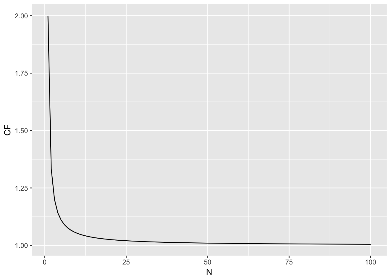
Figure 18.1: Magnitude of the correction factor for small sample size estimations as a function of N.
18.3 Samples from Several Locales
In addition to problems associated with estimating allele freqeuncies incorrectly (and requiring a sample size correction), when we estimate data from several locations, we also have a problem assocaited with the subset of locales relative to the total popualtion size, resulting in a furhter correction to account of the several biased samples you are taking.
\[ H_S = \frac{\tilde{N}}{\tilde{N}-1}\left[ 1 - \sum_{i=1}^\ell \frac{p_i^2}{K} - \frac{H_O}{2\tilde{N}} \right] \]
where \(\tilde{N}\) is the harmonic mean number of genotypes sampled across each of the \(K\) strata. Notice here I use the term \(H_S\) instead of \(H_E\) so that there isn’t any doubt about the differences when we write and talk about these parameters. This formulation (after Nei 1987) corrects for the sampling across separate locations. To indicate that your estimate is being made using subdivided groups of samples, pass the stratum= parameter to genetic_diversity() and set `mode=“Hes”. We can see the magnitude of the correction by looking at a single population and comparing the estimates of \(H_S\) for corrected and non-corrected parameters.
pops <- arapat[ arapat$Population %in% c("32","101","102"),]
he <- genetic_diversity( pops, mode="He")
hes <- genetic_diversity(pops, stratum="Population", mode="Hes")[1:8,]
df <- data.frame(Locus=he[,1], He=he[,2], Hes=hes[,2])
df
## Locus He Hes
## 1 LTRS 0.38850309 0.41230882
## 2 WNT 0.03277778 0.01843238
## 3 EN 0.50285714 0.44289781
## 4 EF 0.27119377 0.31900021
## 5 ZMP 0.09500000 NA
## 6 AML 0.53854875 0.68269231
## 7 ATPS 0.25038580 0.27105726
## 8 MP20 0.80670340 0.81562830They are pretty close (Pearson’s \(\rho =\) 0.970), even when there are only 36 individuals in the sample.2 But they are off and this is a vitally important distinction because if you do not account for these differences you will percolate these errors up through your subsequent analyses (and this is a bad thing).
18.4 Multilocus Diversity
There are several measures of individual locus diversity but few for multilocus diversity. One potential measure for diversity across loci is to based upon the fraction of population that has unique multilocus genotypes. This is defined as:
\[ D_m = \frac{N_{unique}}{N} \]
and can be estimated using the function mulitlocus_diversity(). Looking across the putative species indicated in the data set, we can see that in general, the Cape populations are much less diverse than those individuals samples throughout Baja California.
multilocus_diversity( arapat[ arapat$Species=="Cape",])## [1] 0.56multilocus_diversity( arapat[ arapat$Species=="Mainland",] )## [1] 0.9722222multilocus_diversity( arapat[ arapat$Species=="Peninsula",] )## [1] 0.9007937This is a pretty crude measurement but later when we examine models based upon conditional multilocus genetic distances, we need to make sure that the samples are both allelic rich and multilocus diverse and this approach is a nice way to do that.
The
NAin the \(H_{ES}\) parameter is because there are no smaples in one of the populations and a harmonic mean with a zero in it results in a divide-by-zero error.↩