class: left, bottom background-image: url("images/contour.png") background-position: right background-size: auto # R Data Literacy ### Putting the .box-yellow[Fun] <br/>in Functional Programming [Dr. Rodney J. Dyer](https://dyerlab.org) <p>&nbsp;</p> <p>&nbsp;</p> <img src="images/logo1.svg" width="400px"> --- class: sectionTitle # Rationale --- # Analytical Platforms - Old School .pull-left[ - Mastery required *a priori* - Limitless (mostly) - Steep learning curve ] .pull-right[  ] --- # Slightly less 'Old School' .pull-left[ 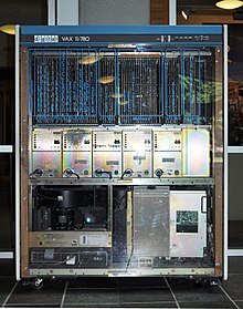 ### SAS on VAX ] -- .pull-right[ ### Greenbar printout for days!!! 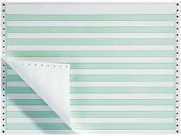 ] --- # Analytical Platforms - Point & Click .pull-left[ - Mastery through discovery (*what does this do?) - Only supporting the most common implementations - Expansion boundaries - Tied to closed-source corporation ] .pull-right[ 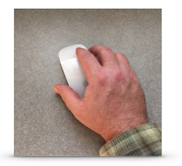 ] --- # Analytical Platforms - Analytical Languages .pull-left[ - Generalized Tools - Expandable by the User - Lower "barrier to entry" - Useful across many domains. ] .pull-right[ 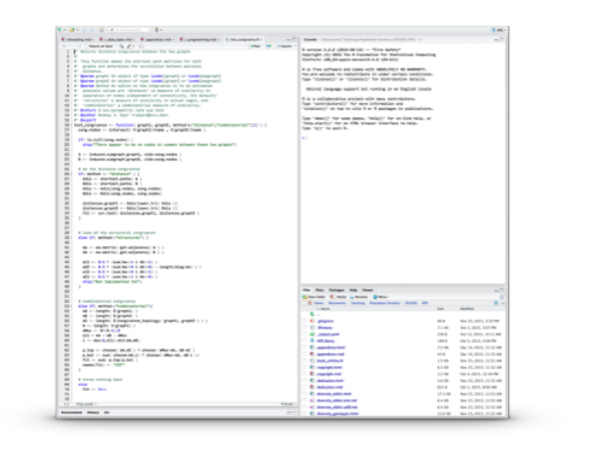 ] --- class: sectionTitle # Why Analytical Languages --- class: center middle  --- class: center middle 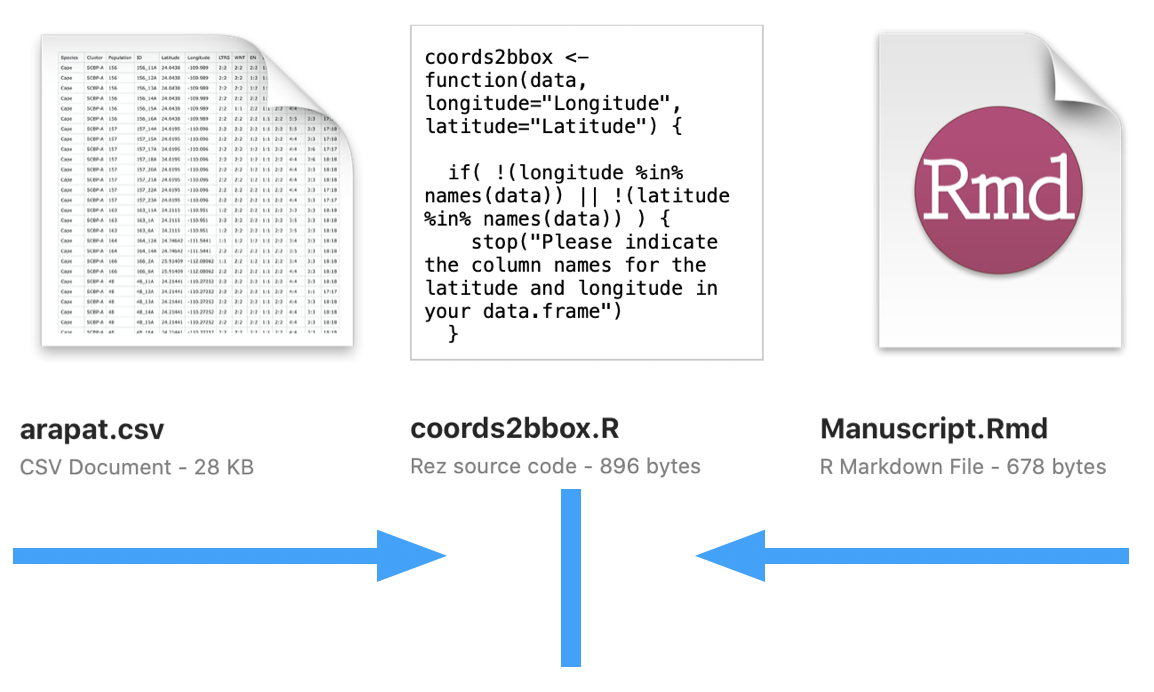 --- class: middle, center <div id="htmlwidget-12b3881e1f70c3f879ba" style="width:100%;height:auto;" class="datatables html-widget"></div> <script type="application/json" data-for="htmlwidget-12b3881e1f70c3f879ba">{"x":{"filter":"none","vertical":false,"data":[["1","2","3","4","5","6","7","8","9","10","11","12","13","14","15","16","17","18","19","20","21","22","23","24","25","26","27","28","29"],["12","153","157","159","160","161","162","163","166","168","171","173","175","177","32","48","51","58","64","73","75","77","84","88","89","9","93","Aqu","Const"],[-112.66552,-110.46236,-110.096,-113.31609,-112.52959,-112.986,-112.408,-110.951,-112.08062,-111.21563,-113.18263,-112.86985,-113.48973,-113.99141,-109.327,-110.27252,-111.60056,-111.35475,-111.32638,-109.85071,-110.74599,-110.69175,-113.66787,-114.29353,-113.39991,-113.94486,-112.04613,-110.10429,-111.675],[27.18232,24.13389,24.0195,27.52944,27.40498,27.0367,27.2028,24.2115,25.91409,25.55757,28.22308,28.40846,28.72796,28.66056,26.63783,24.21441,25.34819,26.0155,25.60521,24.00789,24.58843,24.87611,28.96651,29.32541,28.03661,29.01457,26.94589,23.2855,25.0247],[24,35,26,22,48,64,57,21,19,28,38,19,13,49,40,18,9,11,16,11,16,19,13,23,18,11,25,12,18],[21,41,30,15,36,63,41,21,26,25,39,32,8,50,27,27,11,9,19,5,18,16,17,18,19,10,21,9,11],[0.35190499,0.73248702,0.88102901,0.18796501,0.36519101,0.27910501,0.6136198,0.43287301,0.26730299,0.496464998,0.461356998,0.524267018,0.42144001,0.26179001,0.0562845,0.619518995,0.412512004,0.901878,0.28762299,0.145523,0.8656099,0.422609001,0.395346999,0.218594,0.397500008,0.5641302,0.162724,0.721700013,0.174438]],"container":"<table class=\"display\">\n <thead>\n <tr>\n <th> <\/th>\n <th>Site<\/th>\n <th>Longitude<\/th>\n <th>Latitude<\/th>\n <th>Males<\/th>\n <th>Females<\/th>\n <th>Suitability<\/th>\n <\/tr>\n <\/thead>\n<\/table>","options":{"columnDefs":[{"className":"dt-right","targets":[2,3,4,5,6]},{"orderable":false,"targets":0}],"order":[],"autoWidth":false,"orderClasses":false}},"evals":[],"jsHooks":[]}</script> --- # Linking Data & Narrative The spatial distribution of `\(N =\)` 1408 individuals were sampled from `\(K =\)` 29 sampling sites covering the entire known extent for *Araptus attenuatus* (Figure 2). The observed sex ratio (Females:Males) within each of the sampling locales varied considerably, ranging from a low of 0.455 to 1.68. -- ### 👇🏼 Acutal R Code + Narriative + Analysis Output ```r model <- glm( (Females / Males) ~ log(Suitability), data = araptus, family = Gamma() ) res <- summary(model) ``` Female beetles seem to be selecting locales in more suitable habitats (Figure `\ref{fig-habitat}`), which is consistent with a Gaussian log normal distribution (GLM; intercept = `res$coefficients[1,1]`; coef =` res$coefficients[2,1]`; P =` res$coefficients[2,4]`; Figure `\ref{fig-glm}`). This suggests that males who establish brood chambers at the margins of the species niche are actively selected against by maturing females. --- # Geospatial .pull-left[ <div id="htmlwidget-fc5bbb0f8d2f7c10be27" style="width:504px;height:504px;" class="leaflet html-widget"></div> <script type="application/json" data-for="htmlwidget-fc5bbb0f8d2f7c10be27">{"x":{"options":{"crs":{"crsClass":"L.CRS.EPSG3857","code":null,"proj4def":null,"projectedBounds":null,"options":{}}},"calls":[{"method":"addProviderTiles","args":["Stamen.TerrainBackground",null,null,{"errorTileUrl":"","noWrap":false,"detectRetina":false}]},{"method":"addCircleMarkers","args":[[27.18232,24.13389,24.0195,27.52944,27.40498,27.0367,27.2028,24.2115,25.91409,25.55757,28.22308,28.40846,28.72796,28.66056,26.63783,24.21441,25.34819,26.0155,25.60521,24.00789,24.58843,24.87611,28.96651,29.32541,28.03661,29.01457,26.94589,23.2855,25.0247],[-112.66552,-110.46236,-110.096,-113.31609,-112.52959,-112.986,-112.408,-110.951,-112.08062,-111.21563,-113.18263,-112.86985,-113.48973,-113.99141,-109.327,-110.27252,-111.60056,-111.35475,-111.32638,-109.85071,-110.74599,-110.69175,-113.66787,-114.29353,-113.39991,-113.94486,-112.04613,-110.10429,-111.675],10,null,null,{"interactive":true,"className":"","stroke":true,"color":"#fff","weight":1,"opacity":0.5,"fill":true,"fillColor":"#fff","fillOpacity":0.2},null,null,null,null,null,{"interactive":false,"permanent":false,"direction":"auto","opacity":1,"offset":[0,0],"textsize":"10px","textOnly":false,"className":"","sticky":true},null]},{"method":"addMarkers","args":[[27.18232,24.13389,24.0195,27.52944,27.40498,27.0367,27.2028,24.2115,25.91409,25.55757,28.22308,28.40846,28.72796,28.66056,26.63783,24.21441,25.34819,26.0155,25.60521,24.00789,24.58843,24.87611,28.96651,29.32541,28.03661,29.01457,26.94589,23.2855,25.0247],[-112.66552,-110.46236,-110.096,-113.31609,-112.52959,-112.986,-112.408,-110.951,-112.08062,-111.21563,-113.18263,-112.86985,-113.48973,-113.99141,-109.327,-110.27252,-111.60056,-111.35475,-111.32638,-109.85071,-110.74599,-110.69175,-113.66787,-114.29353,-113.39991,-113.94486,-112.04613,-110.10429,-111.675],{"iconUrl":{"data":"data:image/png;base64,iVBORw0KGgoAAAANSUhEUgAAAAEAAAABCAQAAAC1HAwCAAAAC0lEQVR4nGP6zwAAAgcBApocMXEAAAAASUVORK5CYII=","index":0},"iconWidth":1,"iconHeight":1},null,null,{"interactive":true,"draggable":false,"keyboard":true,"title":"","alt":"","zIndexOffset":0,"opacity":1,"riseOnHover":false,"riseOffset":250},null,null,null,null,["12","153","157","159","160","161","162","163","166","168","171","173","175","177","32","48","51","58","64","73","75","77","84","88","89","9","93","Aqu","Const"],{"interactive":false,"permanent":true,"direction":"center","opacity":1,"offset":[0,0],"textsize":"10px","textOnly":true,"className":"","sticky":true},null]}],"limits":{"lat":[23.2855,29.32541],"lng":[-114.29353,-109.327]}},"evals":[],"jsHooks":[]}</script> ] .pull-right[ ## Quick Visualizations R is the .box-grey[inverse] of ArcGIS. &nbsp; - In ArcGIS, you look at the map and then have to drill down to get to parts of the dataset. &nbsp; - In R, you start with the data and make a map if you want to visualize some aspect of the data. ] --- # Visualizations .pull-left[ <img src="slides_files/figure-html/unnamed-chunk-4-1.png" width="504" /> ] -- .pull-right[ ### Grammar of Graphics ```r araptus %>% ggplot( aes(Suitability, (Females / Males)) ) + geom_smooth(formula = y ~ log(x), method=glm, se=FALSE, color="red", size=0.5) + geom_point() + xlab("Habitat Suitability") + ylab("Observed Sex Ratio (F/M)") + xlim( c(0,1) ) + ylim(c(0.25,1.75)) ``` ] --- class: middle, center 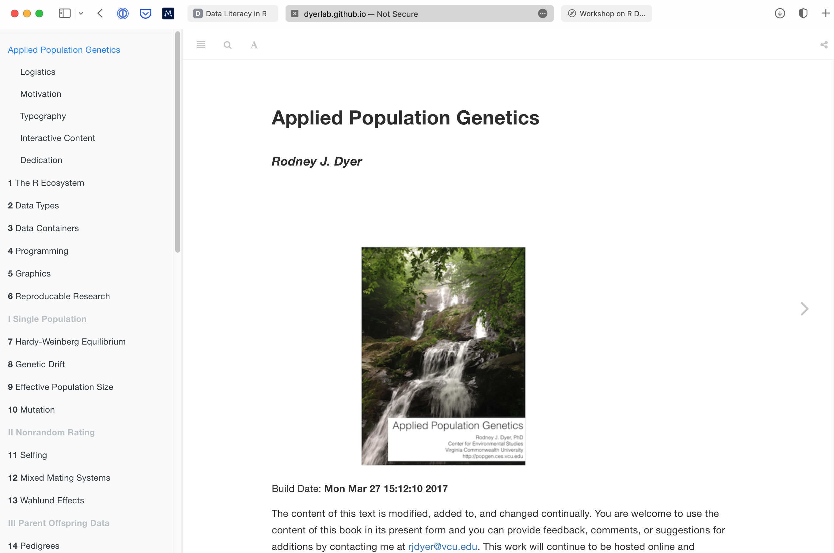 --- # Getting R The canonical location for R is [CRAN](https://cran.r-project.org), which is the main site but has [mirrors](https://cran.r-project.org/mirrors.html) sites located across the world. - Pick a site in close geospatial proximity to you. - Download the installer for your platform (Mac, Windows, Linux) - Follow the instructions on the installer for your particular platform. --- # Sufficent R Version? If you already have R installed on your computer, you may want to make sure it is up-to-date. The last time these slides were compiled (they are written in R as well), the version was: ```r version$version.string ``` ``` ## [1] "R version 4.1.2 (2021-11-01)" ``` To ensure you are able to complete all the activities in this class, please have at least this version on your computer. --- # Keeping Updated If you have a relatively recent version, we can make sure that the packages you already have are also updated by giving the following command. ```r update.packages(ask=FALSE) ``` --- class: sectionTitle # Interacting with R --- class: center middle # The Native `R` Interface 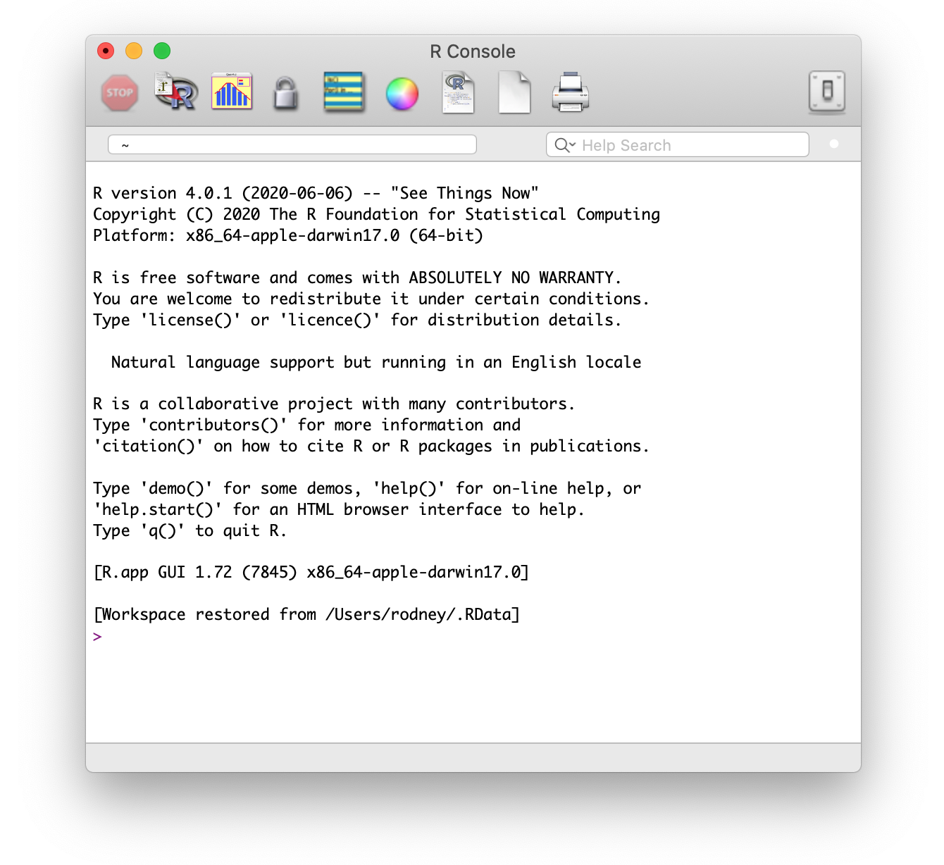 --- class: center middle # R Via the Terminal 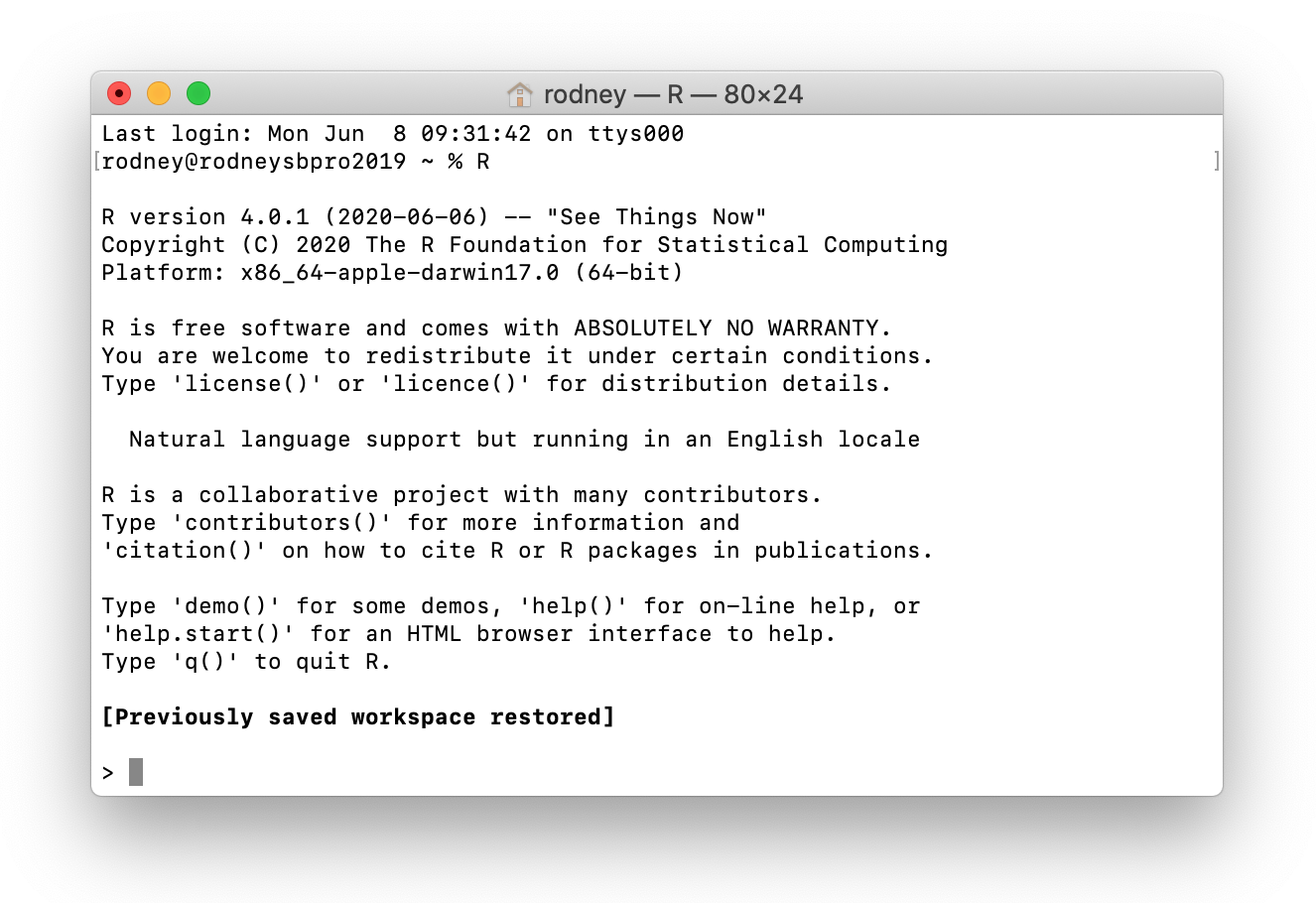 --- class: sectionTitle # RStudio --- # Using RStudio Cloud [RStudio.cloud](https://rstudio.cloud) --- # Tour of the Interface RStudio is essentially a 4-paned browser. --- ## 15 Minute Activity &nbsp; 1. Explore RStudio: Open up `Tools → Global Options` and look through the various panes to familiarize yourself.<br/><br/><br/> 2. Change `General → Save Workspace to .RData on exit` to .red[NEVER] & uncheck `Restore .RData into workspace at startup` <br/><br/><br/> 3. In the `Pane Layout` options, set the top left to **Source** and the top right to **Console** <br/><br/><br/> 4. Explore the `Appearance` options and change the editor theme to suit your own tastes. --- # Projects - Data Integrity .pull-left[ One of the .red[most] important objectives for all analysts. - Localization of data - Consolidation of analyses - Promotes reuse of code - Reproducibility of output ] -- .pull-right[ `RStudio` uses the notion of *Projects*: - Localized on the operating system. - Quick switching between projects. - Customized settings (database connections, etc.) ] --- # 5 Minute Activity - Create Workshop Project 1. `File -> New Project` 2. Select `New Directory` 3. Select `New Project` 4. Place it in a **logical** place on your machine. 5. Move *all of your data sets* into this folder. --- class: sectionTitle # Usage Modality: Console vs. Files --- # Different Functions .pull-left[ The .red[console] is great for interacting directly with `R` for: - Quick operations - Prototyping - Refactoring operations - The Console is externally verbose ] -- .pull-right[ `R` can read input from different kinds of .red[files]: - Script files (.R) contain *pure* code. - Markdown documents (.Rmd) *mix* code and narrative together. - Reports (to pdf, docx, docbook, etc.) - Webpages (e.g., [dyerlab.org](https://dyerlab.org)) - Presentations (e.g., this presentation) - Data Dashboards - Interactive Notebooks (.Rmd) ] --- class: center, middle # Demo Data Localization -- Did you tell them about directionality? --- # Choice of Modality &nbsp; **Console** - When you have quick operations to do. &nbsp; -- **R Script** - When you are only code and/or functions to make, which may be called elsewhere (console or files). &nbsp; -- **Markdown** - When you are creating a narrative around data. --- class: middle background-image: url("images/contour.png") background-position: right background-size: auto .center[ # Questions?  ] <p>&nbsp;</p> .bottom[ If you have any questions for about the content presented herein, please feel free to [submit them to me](https://docs.google.com/forms/d/e/1FAIpQLScrAGM5Zl8vZTPqV8DVSnSrf_5enypyp0717jG4PZiTlVHDjQ/viewform?usp=sf_link) and I'll get back to you as soon as possible.]