The Dyer Laboratory: Simulating Random Populations

Rodney Dyer

The gstudio package has routines that can be used to simulate random populations. I’ve added these to facilitate more exploratory data analysis. Here is how you can use them.

If you have not updated the gstudio and popgraph packages in a while, you probably should. Here is how (if it asks if you would like to update the other packages, it is probably a good idea to say yes).

devtools::install_github("dyerlab/popgraph")
devtools::install_github("dyerlab/gstudio")

Then load it in as:

library(gstudio)

I’m going to start with the enigmatic bark beetle data set.

data(arapat)
summary(arapat)

      Species      Cluster      Population        ID     
 Cape     : 75   CBP-C :150   32     : 19   101_10A:  1  
 Mainland : 36   NBP-C : 84   75     : 11   101_1A :  1  
 Peninsula:252   SBP-C : 18   Const  : 11   101_2A :  1  
                 SCBP-A: 75   12     : 10   101_3A :  1  
                 SON-B : 36   153    : 10   101_4A :  1  
                              157    : 10   101_5A :  1  
                              (Other):292   (Other):357  
    Latitude       Longitude          LTRS          WNT     
 Min.   :23.08   Min.   :-114.3   01:01 :147   03:03  :108  
 1st Qu.:24.59   1st Qu.:-113.0   01:02 : 86   01:01  : 82  
 Median :26.25   Median :-111.5   02:02 :130   01:03  : 77  
 Mean   :26.25   Mean   :-111.7                02:02  : 62  
 3rd Qu.:27.53   3rd Qu.:-110.5                03:04  :  8  
 Max.   :29.33   Max.   :-109.1                (Other): 15  
                                               NA's   : 11  
       EN           EF          ZMP           AML           ATPS    
 01:01  :225   01:01 :219   01:01 : 46   08:08  : 51   05:05  :155  
 01:02  : 52   01:02 : 52   01:02 : 51   07:07  : 42   03:03  : 69  
 02:02  : 38   02:02 : 90   02:02 :233   07:08  : 42   09:09  : 66  
 03:03  : 22   NA's  :  2   NA's  : 33   04:04  : 41   02:02  : 30  
 01:03  :  7                             07:09  : 22   07:09  : 14  
 (Other): 16                             (Other):142   08:08  :  9  
 NA's   :  3                             NA's   : 23   (Other): 20  
      MP20    
 05:07  : 64  
 07:07  : 53  
 18:18  : 52  
 05:05  : 48  
 05:06  : 22  
 (Other):119  
 NA's   :  5

To simulate random data sets we need to start off by determining what allele frequencies you may want. I’m going to use the stratum-level frequencies from the example data set. Here is what these look like.

suppressPackageStartupMessages( library(tidyverse) )
library(DT)
freqs <- frequencies(arapat, stratum="Population")
head(freqs)

  Stratum Locus Allele Frequency
1     101  LTRS     01 0.2777778
2     101  LTRS     02 0.7222222
3     101   WNT     01 1.0000000
4     101    EN     01 0.6111111
5     101    EN     03 0.3888889
6     101    EF     01 0.7142857

though the whole data set has 700 rows!

What I’m going to do is to create a random dataset from these frequencides. This dataset will have 20 populations (I’ll just grab the first 20 Stratum from this frequency matrix).

freqs %>%
  filter( Stratum %in% unique(freqs$Stratum)[1:20] ) -> sim_freqs
summary(sim_freqs)

   Stratum             Locus              Allele         
 Length:370         Length:370         Length:370        
 Class :character   Class :character   Class :character  
 Mode  :character   Mode  :character   Mode  :character  
                                                         
                                                         
                                                         
   Frequency     
 Min.   :0.0500  
 1st Qu.:0.1500  
 Median :0.3500  
 Mean   :0.4297  
 3rd Qu.:0.7000  
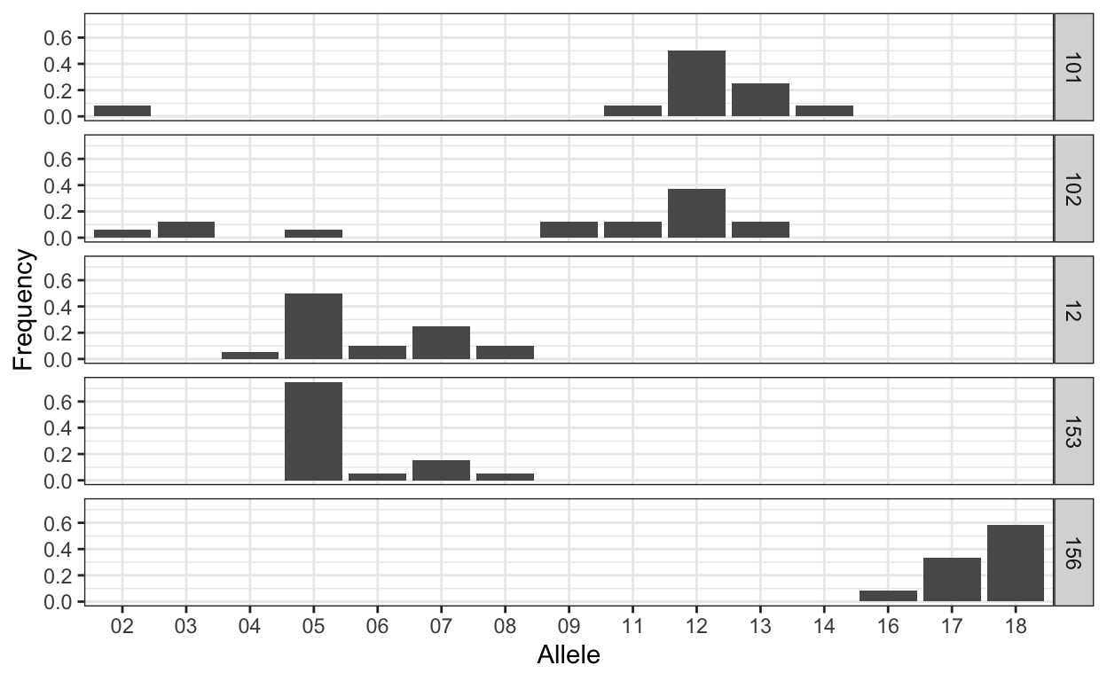
 Max.   :1.0000

And we can take a quick look at the frequencies across populations for, say MP20 as:

sim_freqs %>%
  filter( Locus == "MP20", Stratum %in% unique(Stratum)[1:5] ) %>% 
  ggplot( aes(Allele,Frequency)) + 
  geom_bar( stat="identity", position="dodge" )  + 
  facet_grid( Stratum ~ .) + 
  theme_bw()

OK. Now, lets take a look at how we can make a random population. The make_population() function takes a frequency matrix and creates random individuals. Here is an example.

fake101 <- make_population( sim_freqs %>% filter(Stratum=="101"), N=100 )
head(fake101)

  Population ID   AML  ATPS    EF    EN  LTRS  MP20   WNT   ZMP
1        101  1 08:11 02:09 01:01 01:03 01:01 12:13 01:01 01:01
2        101  2 11:11 02:02 01:01 01:03 02:02 12:13 01:01 01:01
3        101  3 08:08 02:09 01:02 01:03 01:02 12:13 01:01 01:01
4        101  4 08:11 02:09 01:02 01:03 01:01 12:13 01:01 01:01
5        101  5 11:11 02:02 02:02 03:03 01:02 13:14 01:01 01:01
6        101  6 11:11 02:09 01:01 01:01 02:02 02:12 01:01 01:01

The frequencies should be pretty close to the real ones. Compare the LTRS locus allele frequencies from the simualted data

frequencies( fake101,loci = "LTRS")

  Locus Allele Frequency
1  LTRS     01      0.28
2  LTRS     02      0.72

and the real data

sim_freqs %>% filter(Locus=="LTRS", Stratum=="101")

  Stratum Locus Allele Frequency
1     101  LTRS     01 0.2777778
2     101  LTRS     02 0.7222222

Pretty close. So using this approach, we can make all kinds of allele random populations. You just need to figure out the allele frequency matrix and then pass that to the appropriate functions.

Simulating Random Populations

Citation