This is going to require the rayshader library to get some orthorgraphic imagery of topologies. This will be a quick
Install Packages If Necessary
for( lib in c("rayshader","magick") ) {
  if( !require(lib) ) {
    install.packages(lib)
  }
}

if( !require(webshot2 ) ) {
  remotes::install_github("rstudio/webshot2")
}
The Data
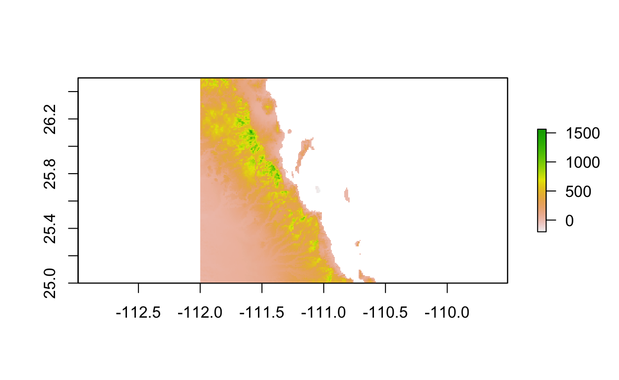
For this example, I’m going to use a section of Baja California, in the vacinity of the town of Loreto, BCS.

We can load it in using the direct url and crop it to the approximate size of the area of interest.
I have a raster up on github for my teaching site that we’ll use.
url <- "https://github.com/dyerlab/ENVS-Lectures/raw/master/data/alt_22.tif"
raster( url ) %>%
  crop(extent( -112, -110.5, 25, 26.5) ) -> baja_california
plot( baja_california )
Now, we should probably reproject the raster. Right now, the datum for it is defined as:
crs( baja_california )
Coordinate Reference System:
Deprecated Proj.4 representation: +proj=longlat +datum=WGS84 +no_defs
WKT2 2019 representation:
GEOGCRS["WGS 84 (with axis order normalized for visualization)",
    DATUM["World Geodetic System 1984",
        ELLIPSOID["WGS 84",6378137,298.257223563,
            LENGTHUNIT["metre",1]]],
    PRIMEM["Greenwich",0,
        ANGLEUNIT["degree",0.0174532925199433]],
    CS[ellipsoidal,2],
        AXIS["geodetic longitude (Lon)",east,
            ORDER[1],
            ANGLEUNIT["degree",0.0174532925199433,
                ID["EPSG",9122]]],
        AXIS["geodetic latitude (Lat)",north,
            ORDER[2],
            ANGLEUNIT["degree",0.0174532925199433,
                ID["EPSG",9122]]]]
Which is great. However, the x- and y- coordinates in this are defined by degrees, whereas the values in it, the z-axis for us below, is defined in the unit of meters.
Let’s reproject this raster (see lecture here if you want to know more about rasters) to a datum whose units are also in meters. I grabbed the proj.4 definition of epsg = 6366, which covers Mexico west of -114 degrees in zone 11N.
baja_utm <- raster::projectRaster(baja_california, crs="+proj=utm +zone=11 +ellps=GRS80 +towgs84=0,0,0,0,0,0,0 +units=m +no_defs ")
baja_utm
class      : RasterLayer
dimensions : 197, 201, 39597  (nrow, ncol, ncell)
resolution : 838, 926  (x, y)
extent     : 993606.5, 1162044, 2769727, 2952149  (xmin, xmax, ymin, ymax)
crs        : +proj=utm +zone=11 +ellps=GRS80 +units=m +no_defs
source     : memory
names      : alt_22
values     : -202, 1408.906  (min, max)
Before I move on, I’m going to smooth out the jaggedness of this a bit exmaple here.
smooth_utm <- focal( baja_utm,
w = matrix(1, 3, 3),
fun = mean,
na.rm=TRUE)
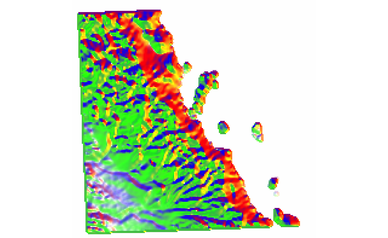
par( mfrow =c(1,2) )
plot( baja_utm, legend=FALSE )
plot( smooth_utm, legend=FALSE )
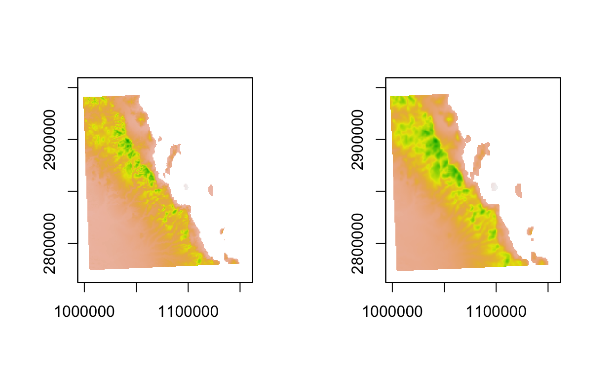
Just taking the ‘edge’ off, so to speak. For some reason, one of the islands is denoted as negative elevation, so I’ll fix that
baja_matrix <- abs( raster_to_matrix( smooth_utm ) )
And then clean it up. This elevation raster was originally provided by WorldClim, which ignores elevations in the water. So there is a ton of NA values for where the Pacific Ocean and Sea of Cortéz is located. I’m going to replace all the NA with 0
Plotting with Shading
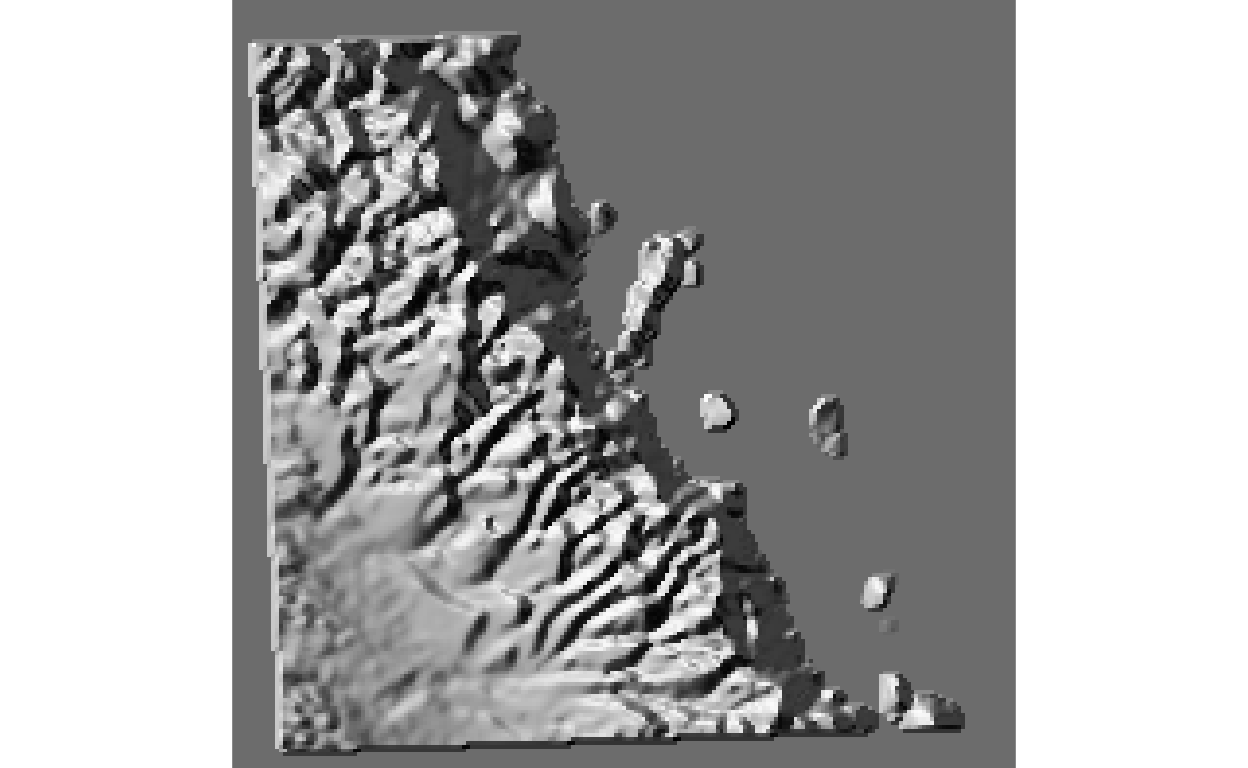
The matrix can now be plot with shading. There are several built-in palettes (and you can supply your own as well).
baja_matrix %>%
  sphere_shade( texture="bw" ) %>%
  plot_map()
The possible values include:
texture > Default ‘imhof1’. Either a square matrix indicating the spherical texture mapping, or a string indicating one of the built-in palettes (‘imhof1’,‘imhof2’,‘imhof3’,‘imhof4’,‘desert’, ‘bw’, and ‘unicorn’).
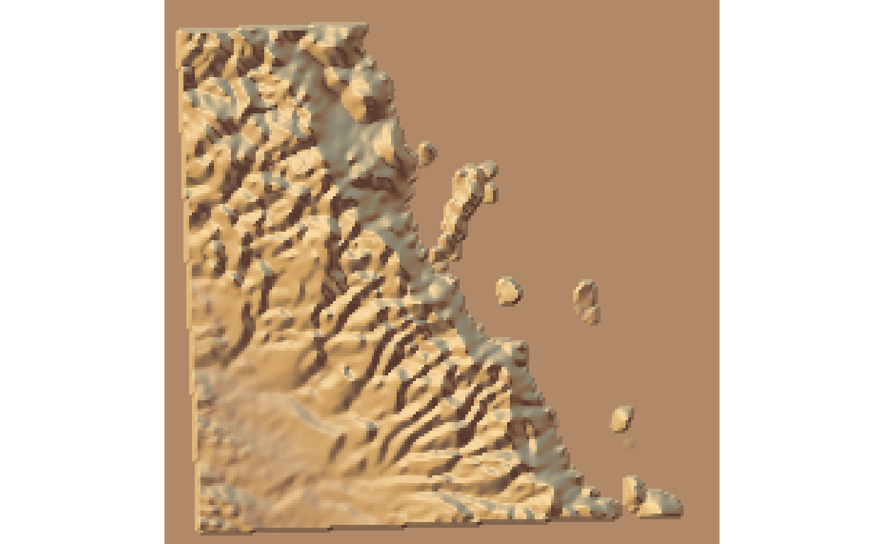
Which look like this
baja_matrix %>%
  sphere_shade( texture = "desert" )  %>%
  plot_map()
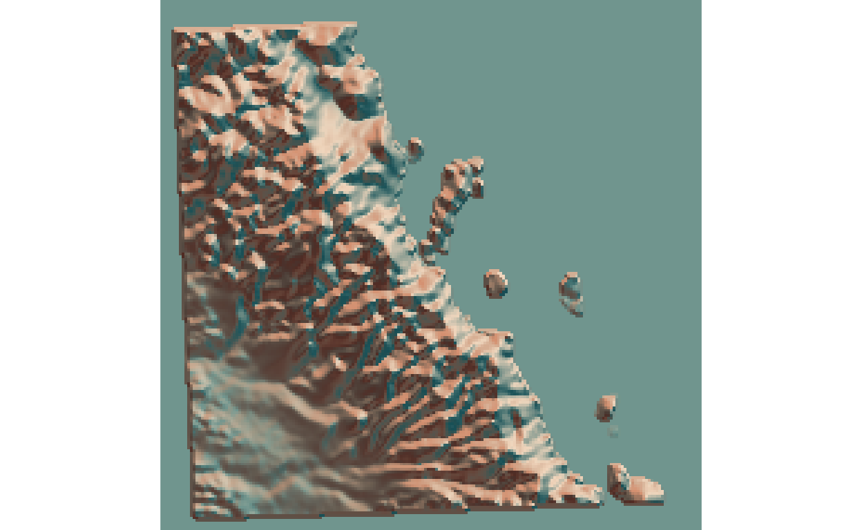
and this
baja_matrix %>%
  sphere_shade( texture = "imhof2",
                sunangle = 45 ) %>%
  plot_map()
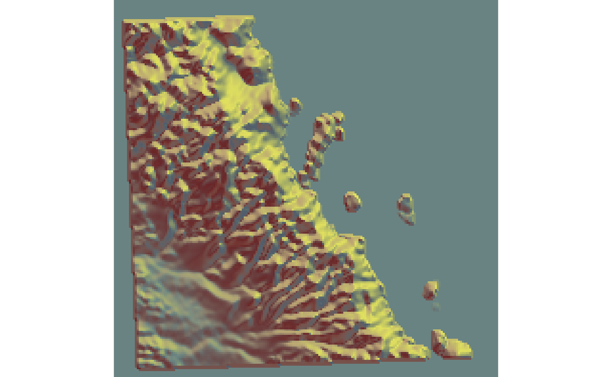
and this.
baja_matrix %>%
  sphere_shade( texture = "imhof3",
                sunangle = 45 ) %>%
  plot_map()
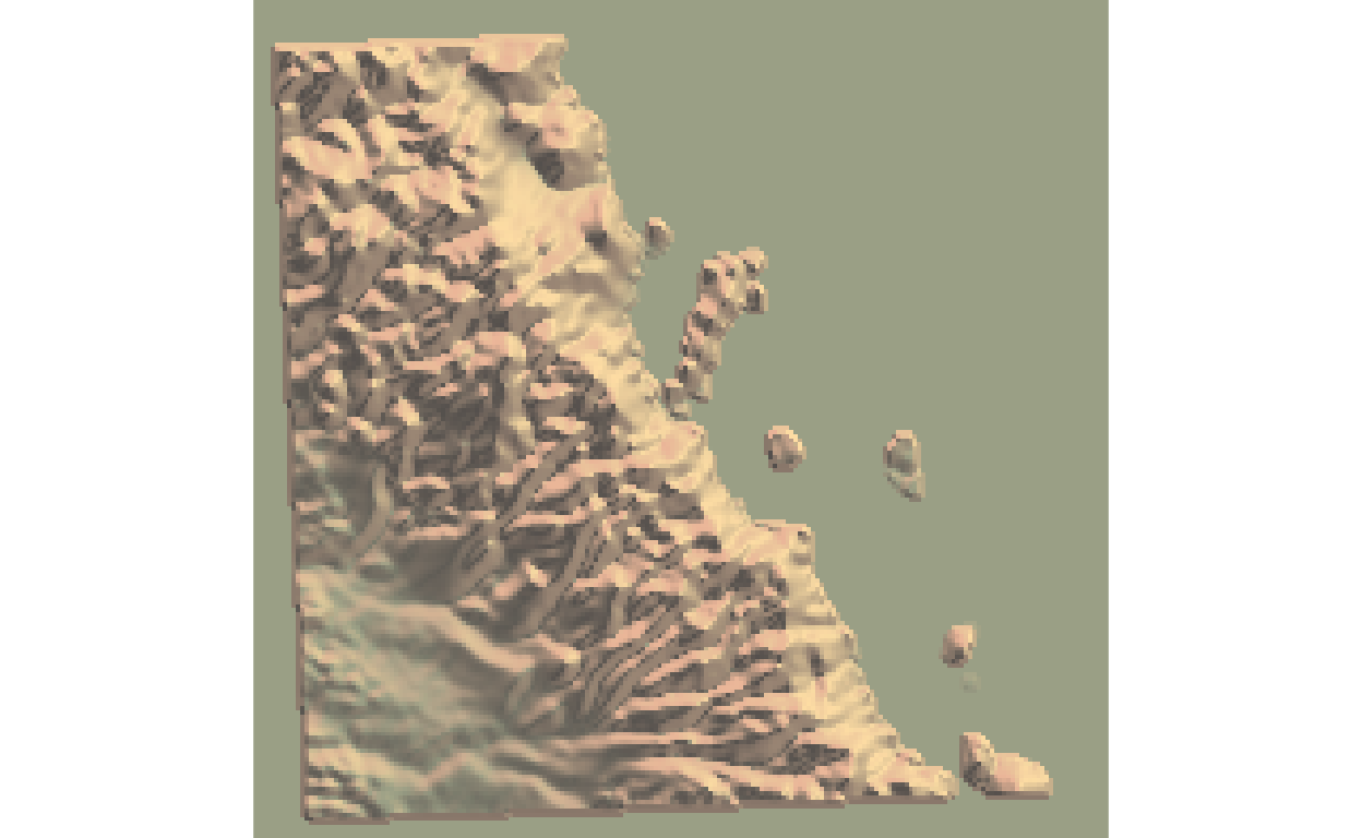
and this
baja_matrix %>%
  sphere_shade( texture = "imhof4",
                sunangle = 45 ) %>%
  plot_map()
and of course, there is a unicorn
baja_matrix %>%
  sphere_shade( texture = "unicorn",
                sunangle = 45 ) %>%
  plot_map()
Adding Water
Water can be represented as either opaque or transparent. These rasters do not have bathymetry data (and I set them all to zero), so I’ll this part and just make it a solid color.
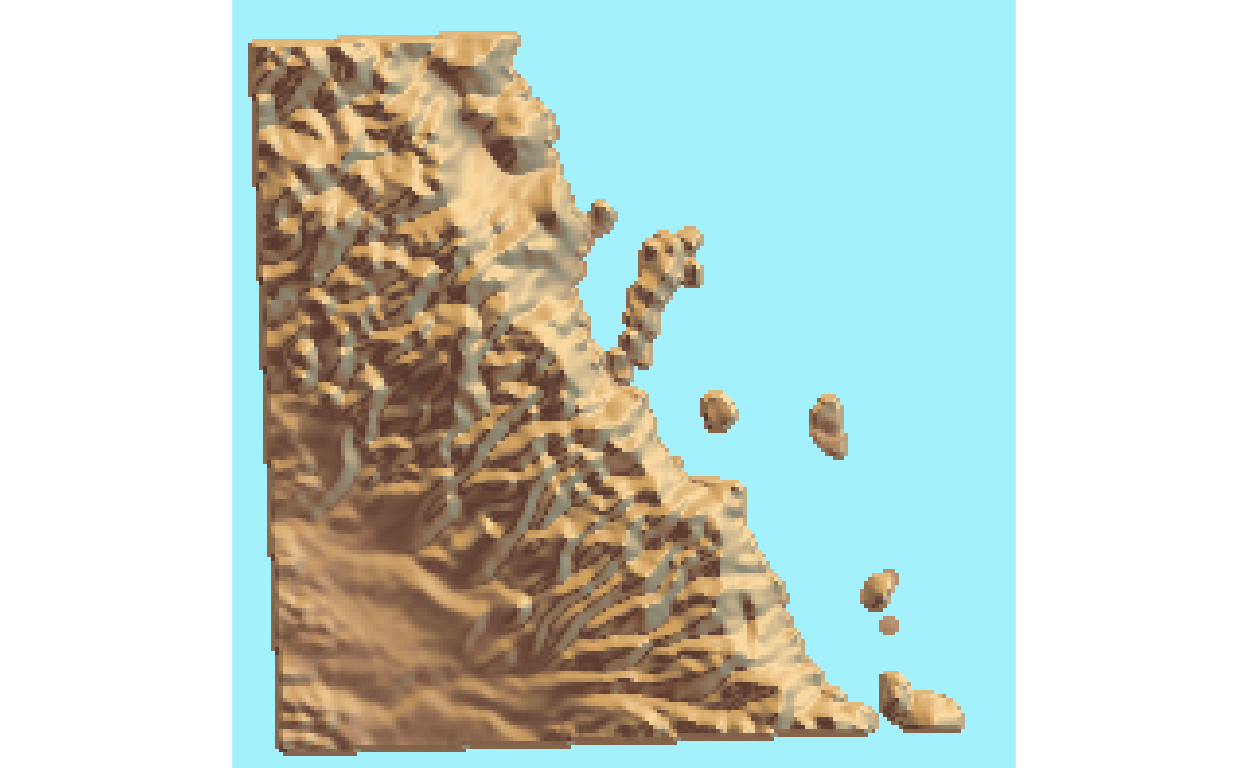
baja_matrix %>%
  sphere_shade( texture = "desert",
                sunangle = 45 ) %>%
  add_water( detect_water( baja_matrix ), color = "desert") %>%
  plot_map()
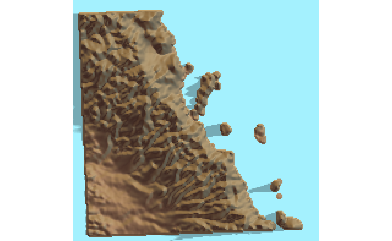
Adding Shadows
There are several different kinds of shadings we can add to a scene. Here I’ll shading from the sun (and setting the angle and altitude).
baja_matrix %>%
  sphere_shade( texture = "desert",
                sunangle = 45 ) %>%
  add_water( detect_water( baja_matrix ), color = "desert") %>%
  add_shadow( ray_shade( baja_matrix,
                         sunangle=82,
                         sunaltitude = 85), 0.5) %>%
  plot_map()
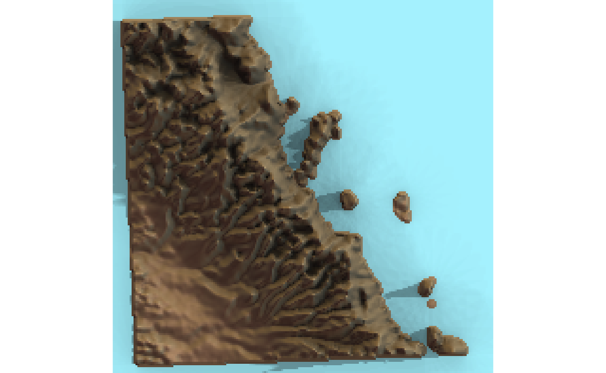
We can also add onto that ambient shading.
baja_matrix %>%
  sphere_shade( texture = "desert",
                sunangle = 45 ) %>%
  add_water( detect_water( baja_matrix ), color = "desert") %>%
  add_shadow( ray_shade( baja_matrix,
                         sunangle=82,
                         sunaltitude = 85), 0.5) %>%
  add_shadow( ambient_shade( baja_matrix), 0 ) %>%
  plot_map()
Rendering in 3-Space
Now let’s make it a bit more interactive. Unfortunately, you will not be able to see the popup window and use your mouse to move it around as this is being cast onto a static webpage (so run the code yourself).
The following steps will require that you can plot rgl content. Depending upon your platform, you may need to download a few things. For example, on OSX, you need to download XQuartz (google it). I have no idea what you’ll need on Windows or Linux.
This will plot it and then render it appropriately in an external window.
baja_matrix %>%
  sphere_shade( texture = "desert",
                sunangle = 45 ) %>%
  add_water( detect_water( baja_matrix ), color = "desert") %>%
  add_shadow( ray_shade( baja_matrix,
                         sunangle=82,
                         sunaltitude = 85), 0.5) %>%
  add_shadow( ambient_shade( baja_matrix), 0 ) %>%
  plot_3d( baja_matrix/5,
           zscale=10,
           fov=0,
           theta = 135,
           zoom = 1,
           phi = 45,
           windowsize = c(1000,800))
Sys.sleep(0.2)
render_snapshot()
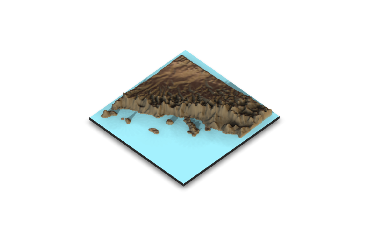
The parameters of plot_3d include: - zscale: scaling in the z-axis. - fov: Field of View. - theta: Rotation of the landscape. - zoom: Zoom
- phi: Angle at which camera is looking at the landscape
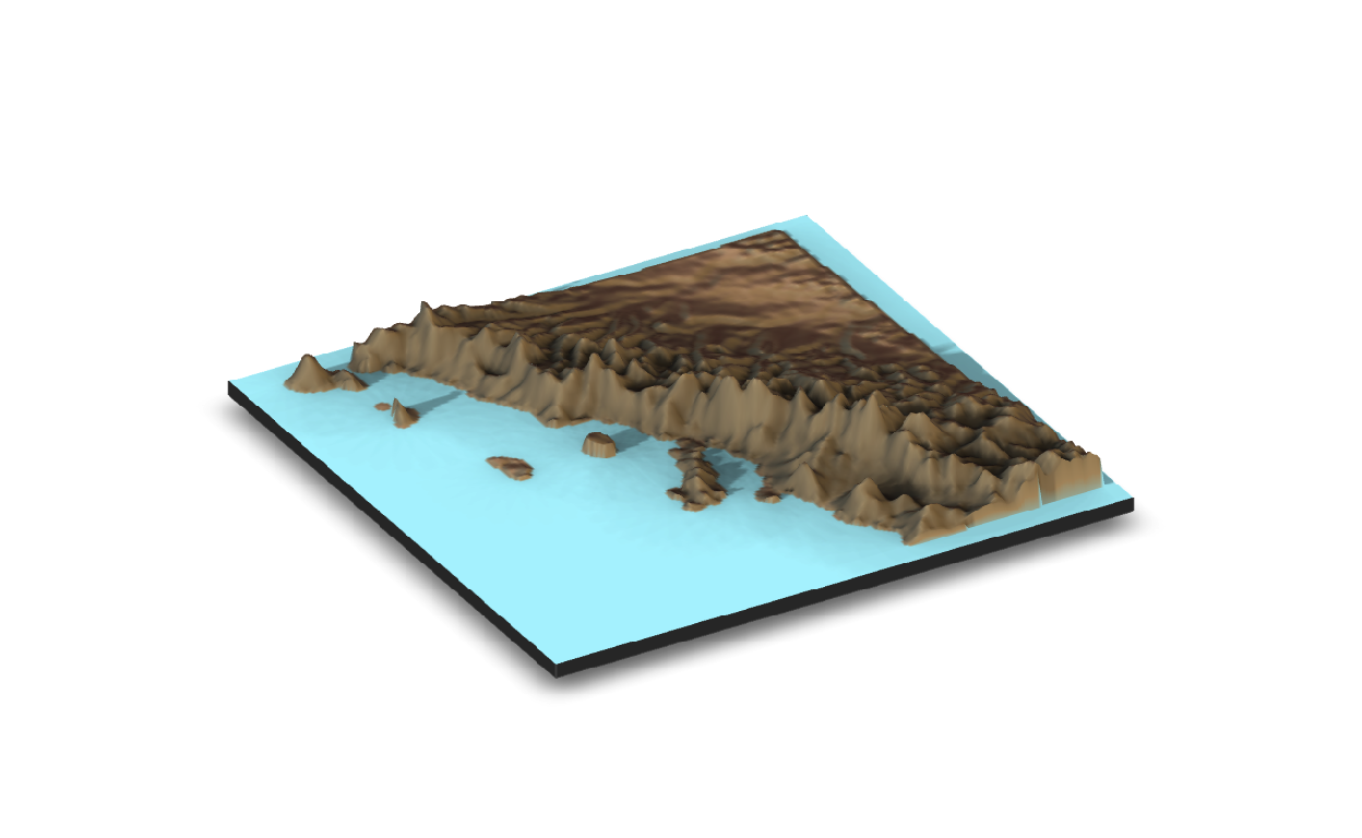
You’ll just have to play around with these to get them to look proper for the landscape you are using.
baja_matrix %>%
  sphere_shade( texture = "desert",
                sunangle = 45 ) %>%
  add_water( detect_water( baja_matrix ), color = "desert") %>%
  add_shadow( ray_shade( baja_matrix,
                         sunangle=82,
                         sunaltitude = 85), 0.5) %>%
  add_shadow( ambient_shade( baja_matrix), 0 ) %>%
  plot_3d( baja_matrix/5,
           zscale=10,
           fov=0,
           theta = 150,
           zoom = 0.75,
           phi = 30,
           windowsize = c(1000,800))
Sys.sleep(0.2)
render_snapshot()
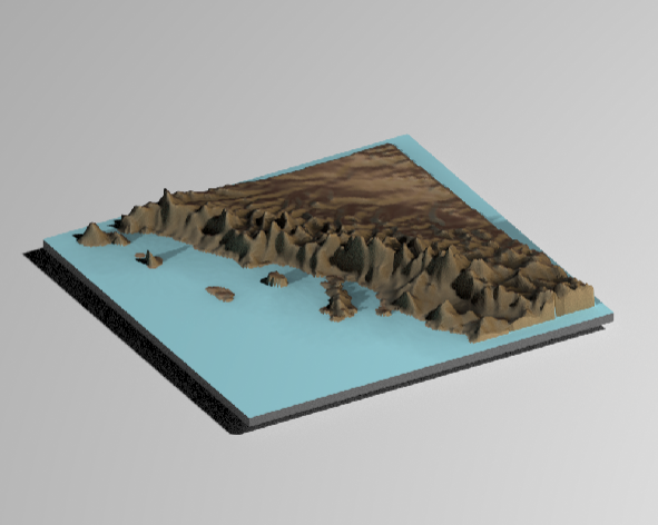
We can even use multi-pass rendering to make the image a bit better in quality.
baja_matrix %>%
  sphere_shade( texture = "desert",
                sunangle = 45 ) %>%
  add_water( detect_water( baja_matrix ), color = "desert") %>%
  add_shadow( ray_shade( baja_matrix,
                         sunangle=82,
                         sunaltitude = 85), 0.5) %>%
  add_shadow( ambient_shade( baja_matrix), 0 ) %>%
  plot_3d( baja_matrix/5,
           zscale=10,
           fov=0,
           theta = 150,
           zoom = 0.75,
           phi = 30,
           windowsize = c(1000,800))
Sys.sleep(0.2)
render_highquality(samples=200, scale_text_size = 24, clear=TRUE)
That looks pretty good for a cheap and quick 3d render.