10 Mutation

Mutation is the ultimate source of genetic variation. If mutation never existed, all our loci would be the same homozygote and all of you would look like me!

Mutation is the process whereby changes are induced into genetic encodings. Without mutation as a process, there would be no genetic variation (and no evolution). In basic terms, we can break mutations into two categories.

Somatic Mutation: A mutation that occurs outside the germline and will not be passed to subsequent generations. Somatic mutations may influence the fitness (survival and reproductive output) of individuals but do not have an effect on the genetic information being passed to offspring.

Germ Line Mutation: A mutation that can be passed to a gamete, resulting in an overall change in population genetic structure. There are several mechanisms that can result in mutations. Mutation as a process occupies a special place in the public vernacular—just look at all the science fiction movies where mutation is the initial arbiter of conflict. Fortunately, these scenarios do not reflect reality.

There are many types of mutations that we can encounter in our data. Much of what we teach about mutations at the undergraduate level has to do with DNA sequences that encode for amino acids, though much of population genetics focuses on genetic markers outside of coding regions. It is illogical to talk about missense, nonsense, or synonymous mutations at a microsatellite locus. For the purposes of this text, we will focus on nucleotides and other common markers.

10.1 Mutation Models

Mutation models are conceptual characterizations of how the process of mutation results in the development of new allelic states. At this stage, I’m going to focus only on the change of the underlying genetic material (e.g., a transition mutation or altering allele A to become allele a) and not consider the fitness consequences of these changes.

No matter how large the population is, with increasing $\mu$, the presence of newly mutated alleles are almost always observed in heterozygotic state.

From a sampling perspective, it is difficult to get a good estimate of the allele frequencies for these rare alleles. Depending upon your research question, this may be a good thing or a bad one. For example, if you are looking at demographic processes, the presence of a rare allele may indicate that historical (or ongoing) gene flow may be an important factor. Conversely, rare alleles (by definition) are not commonly observed, so if there is a ‘marker’ like this, it may be difficult to actually sample without large sampling effort.

Small allele frequencies of newly mutated allele, pi, are more likely to be lost due to genetic drift as the they are more likely to be found as heterozygotes. Only half the offspring are expected to have them and the probability of persistence is proportional to its current allele frequency.

At a two-allele locus, we can model the frequencies for a particular set of data as falling along a line defined by $p+q=1.0$. Consider the three populations in the next figure, who have allele frequencies of f(A) = c(0.15, 0.42, 0.59).

By definition, the allele frequencies define a coordinate in 2-dimensional space for each population. This coordinate space has as many dimensions as there are alleles at the locus, each of them being orthogonal to all the others. For a 2-allele system, they can be represented by a x & y coordinate.

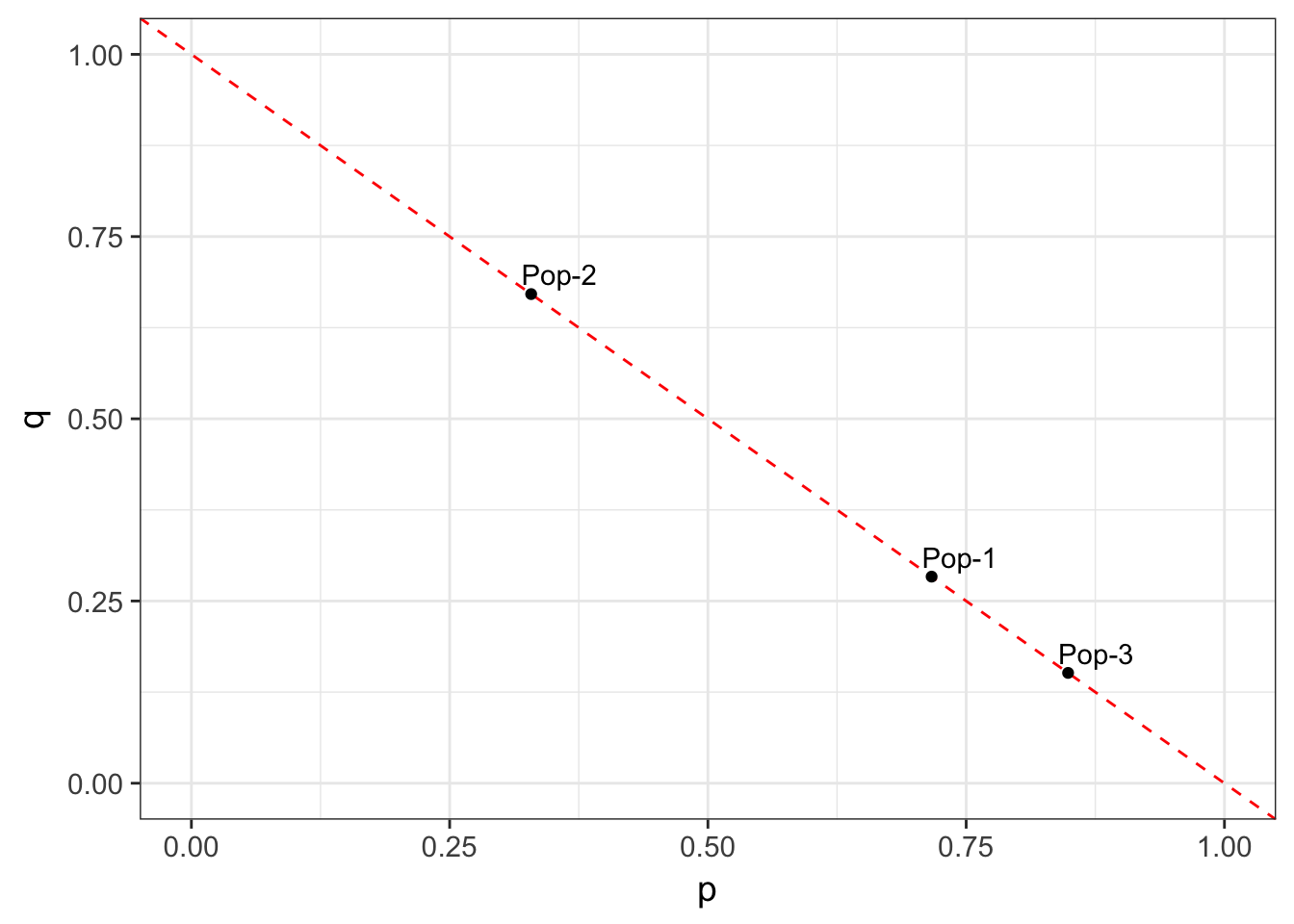
Figure 10.1: Allele frequencies depicted for three different populations. All population frequency spectra must fall on the dotted line.

Three allele loci can be plot in 3-space ($x$, $y$, and $z$ coordinates). Higher number of allele per locus are more problematic to depict on a 2-dimensional image, but the analogy holds.

With an $\ell$-allele locus, we have $\ell-1$ statistically independent alleles. We loose one degree of freedom because the frequencies are under the constraint of $\sum_{i=1}^\ell p_i = 1.0$—all frequencies must sum to unity. Statistically, this approach allows us to consider our individual genotypes as well, as being describe as a matrix with $\ell-1$ statistically independent columns. So, for example, consider the genotypes $AA$, $AB$, $AC$, $BB$, $BC$, $CC$. These genotypes can be encoded in a matrix with 6 rows (one for each individual) and 3 columns (one for each allele). The values inserted into each are the frequency (or alternatively the count) of the alleles in each locus.

\[ X = \begin{bmatrix} 1 & 0 & 0 \\ 0.5 & 0.5 & 0 \\ 0.5 & 0 & 0.5 \\ 0 & 1 & 0 \\ 0 & 0.5 & 0.5 \\ 0 & 0 & 1 \\ \end{bmatrix} \]

In R, we can encode loci

library(gstudio)
loci <- c( locus( c("A","A")), locus( c("A","B")), locus( c("A","C")), locus( c("B","B")), locus( c("B","C")), locus( c("C","C")) )
loci

## [1] "A:A" "A:B" "A:C" "B:B" "B:C" "C:C"

and translate them into multivariate encoded data in the same way.

mv.genos <- to_mv( loci )
mv.genos

##        A   B   C
## [1,] 1.0 0.0 0.0
## [2,] 0.5 0.5 0.0
## [3,] 0.5 0.0 0.5
## [4,] 0.0 1.0 0.0
## [5,] 0.0 0.5 0.5
## [6,] 0.0 0.0 1.0

If you are going to use this as a data matrix for multivariate analyses, you need to drop one of the columns since each column sums to unity. If you do not, you will not be able to invert the matrix because it is singular and essentially the entire universe will cease to exist—ok maybe I’m exaggerating a bit here but inverting singular matrices is not something you want to try. It does not matter which of the columns you drop, some like to drop the most rare allele or the most common one, but it is irrelevant.

to_mv( loci, drop.allele = TRUE )

##        A   B
## [1,] 1.0 0.0
## [2,] 0.5 0.5
## [3,] 0.5 0.0
## [4,] 0.0 1.0
## [5,] 0.0 0.5
## [6,] 0.0 0.0

The reason that I think this is important, in the context of mutation, is that a mutation event can move entries from one column to another (if an allele mutates to anther existing allele) or add additional columns to the matrix (if the mutation produces an allele that was not previously in the data). The dimensionality of the data, for a locus and across loci, is simply the number of independently assorting alleles in the system. Mutation as a process can add additional dimensions (e.g., degrees of freedom in a statistical sense) to the data itself. In the following mutation models, consider the consequences to how these models influence the way in which we denote genotypes and population allele frequencies in a multivariate context.

10.1.1 Fixed Allele Model

The fixed allele model is one where there are a finite number of allelic states. The frequency of the allele, say $f(A) = p$, can estimated across generations if we know the rate at which say the A is mutated to become the other state, say the a allele. For simplicity, lets define this rate as $\mu$, on a per generation basis. Across generations then, it is pretty easy to predict what the frequency of both alleles will be each generation by iterating each generation and estimating the frequencies based upon the previous generation. An example of this is given in the table below, where a locus fixed for the A allele is experiencing mutation at a rate of $\mu=0.001$.

With each successive generation, a fraction of the A alleles are being mutated. Under a fixed allele model, these mutations result in the identity of that allele being one of a fixed number of other alleles. If this were a dual fixed allele model, the mutation rate, $\mu$, would represent the rate of change from $A \to a$. There would also be a corresponding rate in the opposite direction, say $a \to A$ at a per generation rate of $\nu$. The presence of these two alleles (or at least a finite set of defined alleles), who change state due to mutation is the definition of the fixed allele model.

$AA$, $AB$, $AC$, $BB$, $BC$, $CC$.

Once defined, there is a pretty easy set of algebra associated with predicting what the next and subsequent generations of allele frequencies may be based upon mutation rates. Later when we examine migration, we will see a similar approach to estimating allele frequencies so pay attention to both the specifics of the this as well as how we are formulating the equation conceptually.

Assuming a 2-allele system, the frequency of the $A$ allele, denoted as say $p$, in the next $(t+1)$ generation is:

The frequency of the allele at this generation, $p_t$, multiplied by the fraction of individuals who did not mutate from $A \to a$. This can be written as $p_t(1-\mu)$. To this we also add,
The fraction of alleles that were not $A$ at this generation $(1-p_t)$ but who were mutated to the $A$ state during the transition from $t$ to $t+1$. This is written as $(1-p_t)\nu$.

So the frequency at $p_{t+t}$ is:

\[ p_{t+1} = p_t(1-\mu) + (1-p_t)\nu \]

We can plot this relationship through time to visualize how allele frequencies change. Here I start with a relatively high mutation rate of $\mu=0.0075$ ($A \to a$) and $\nu = 0.01$ ($a \to A$) and a starting allele frequency of $p=0.75$. We can set up a ‘simulation’ on these parameters as:

p <- 0.75
mu <- 0.75e-2
nu <- 1e-2
T <- seq(1,3000000,by=5000)
p <- rep( p, length(T) )
for( i in 2:length(T)){
  pt <- p[i-1]
  p[i] <- (1-mu)*pt + (1-pt)*nu
}

Where I create two vectors, one for time, $T$, and the other for the current allele frequency. I then iterate across generations (the for(i in 1:length(t)) ) and for each generation I grab the allele frequencies of the previous generation and use them to estimate the frequency for next generation. After we iterate across all the generations, we can plot the expected allele frequencies through time as:

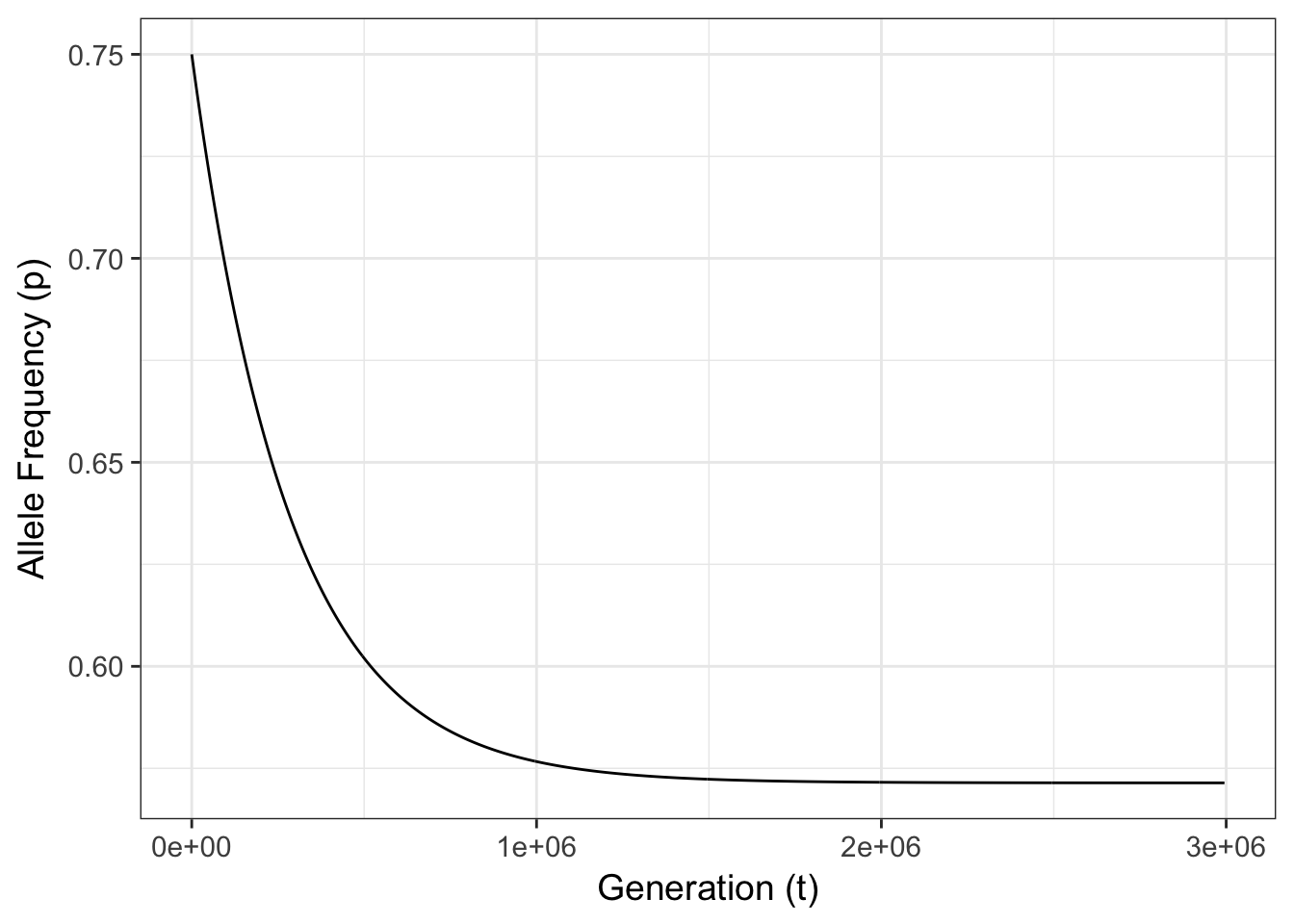
$Expected allele frequencies for a single 2-allele locus with mutation rates of $\mu=0.0075$ and $\nu=0.01$ and a starting allele frequency of $p_0 = 0.75$.$

Figure 10.2: Expected allele frequencies for a single 2-allele locus with mutation rates of $\mu=0.0075$ and $\nu=0.01$ and a starting allele frequency of $p_0 = 0.75$.

There are two things that are of interest in this figure.

Given the values of $\mu$ and $\nu$ the final frequency will change through time tending towards some equilibrium frequency, $\hat{p}$. The rate of change, $\delta p$, is dependent upon how far away the initial allele frequency is from $\hat{p}$ and the difference in the mutation rates, $|\mu - \nu|$.
The consequences of mutation are significantly though exceedingly slow. If you look at the figure, notice the number of generations on the x-axis. It takes somewhere in the vicinity of 500,000 generations for the allele frequency to go from $p=0.75$ to $p=0.60$!

If we set $p_{t+1} = p_t$ (e.g., when there is no change in allele frequencies) and solve for $p$, the previous equation be rearranged to give the equilibrium allele frequencies for the $A$ allele, $\hat{p}$, given the relative values of $\mu$ and $\nu$ as:

\[ \hat{p} = \frac{\nu}{\nu + \mu} \]

Independent of the starting frequencies, all populations will tend towards this equilibrium state (assuming nothing else is happening to the population during all those generations).

The rate of change and the distance away from the equilibrium frequency, $\hat{p}$, can be used to derive an estimate of allele frequencies with mutation at any arbitrary generation. This expectation is:

\[ p_t = \frac{\nu}{\mu + \nu} + \left(p_0 - \frac{\nu}{\mu+\nu} \right)(1 - \mu - \nu)^t \]

If you look at the components of this relationship, it can be decomposed into the following parts.

The destination allele frequency where the population will eventually stabilize at, $\frac{\nu}{\mu + \nu}$,
The distance the starting generation is away from this destination, $\left(p_0 - \frac{\nu}{\mu+\nu} \right)$,
The rate at which the both mutation directions change this frequency, $(1 - \mu - \nu)$,
And the length of time (in generations) that has elapsed since starting at $p_0$, $t$.

This is a pretty standardized construction and we will see a very similar approach when dealing with allele frequency changes due to migration.

10.1.2 Infinite Allele Model

For many genetic components, there is more than just two different states, A and a (despite what we use in teaching population genetics). Kimura & Crow (1964) defined the infinite alleles model. Here, instead of having only two alleles with mutation flipping states of the alleles, the infinite alleles model adds new alleles to the locus with each mutation.

Both the fixed allele model and the infinite allele model can be easily configured in R using the multivariate encoding ‘allele space’ paradigm outlined previously.

10.1.3 Stepwise Mutation Model

Markers such as microsatellite require slightly different mutation models. A microsatellite locus is one where nucleotide motifs are repeated and the length of the fragment containing the repeats (plus some flanking primer sequences) is used as the definition of the allele. Mutation at microsatellite loci is due to the gain or loss of motifs during replication. Mutation models for these kinds of loci incorporate the probability of gain/loss of one or more motifs. Usually, the likelihood of single motif changes are considered more common than events resulting in changing fragment lengths by several motifs at once. This kind of mutation model can be summarized as shown below for changes in allelic state across generations. Later when we examine genetic distance measures, we will return to this metric.

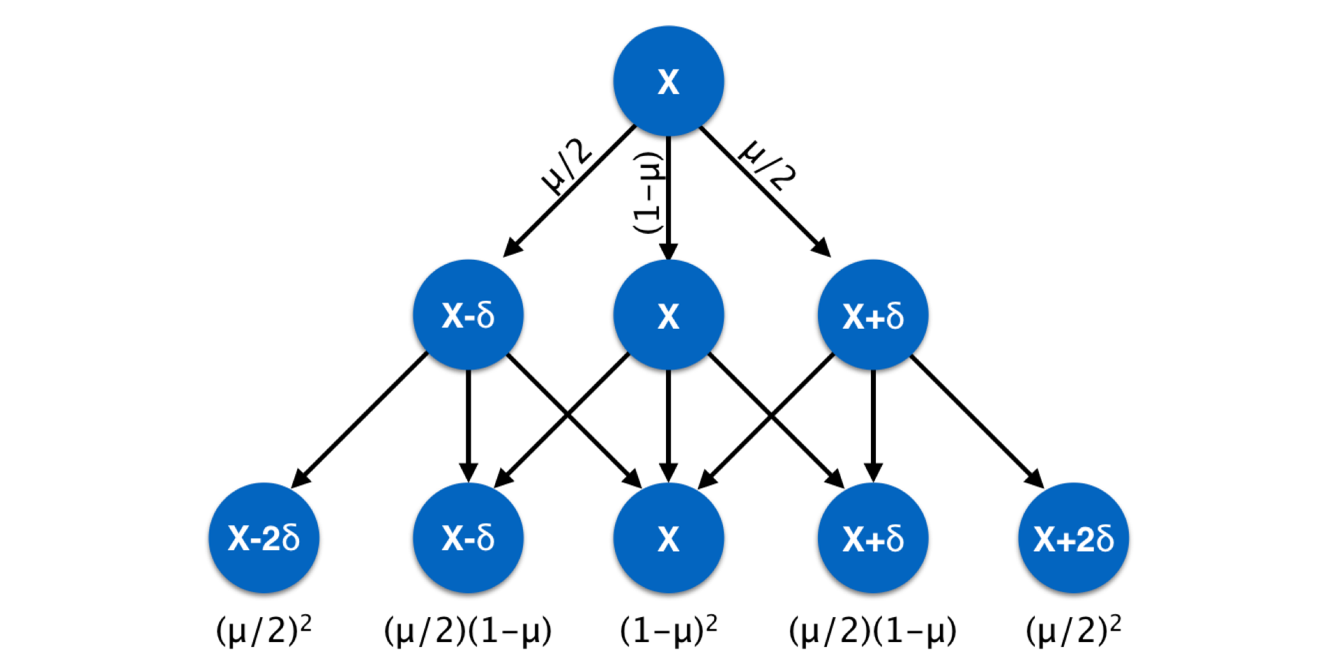
$Schematic of stepwise mutation model across three generations, commonly used in describing changes at microsatellite loci with a repeat motif length of $\delta$ deviating from a mean fragment size.$

Figure 10.3: Schematic of stepwise mutation model across three generations, commonly used in describing changes at microsatellite loci with a repeat motif length of $\delta$ deviating from a mean fragment size.

10.2 Mutation and Inbreeding

Inbreeding, the relative decrease in heterozygosity (or increase in heterozygosity) is influenced by mutation rates because of the way that mutation influences the level of autozygosity.

\[ F_{t+1} = \frac{1}{2N_e} + \left( 1 - \frac{1}{2N_e}\right)F_t \]

where the next generation level of autozygosity is made up of:

$\frac{1}{2N_e}$ is the likelihood that two alleles at a locus are autozygous this generation, and
$\left( 1 - \frac{1}{2N_e} \right)F_t$ is the fraction of homozygous individuals in the previous generation that were autozygous.

From this relationship, we see that $F$ increases most rapidly towards its eventual asymptote with smaller effective population sizes (see Chapter 9).

The presence of mutation in this model breaks up the symmetry by changing the state of alleles delivered to the next generation. For diploid individuals, mutation can occur as depicted in the following table.

Mutant Allele	Frequency
0	$(1-\mu)^2$
1	$2\mu(1-\mu)$
2	$\mu^2$

For any particular locus, a mutation either not occur, occur once, or occur twice. If an individual is $AA$ a mutation changes this genotype to be heterozygous, and by definition, incapable of being autozygous (or even allozygous). A genotype of $AB$, while heterozygous and neither auto- or allozygous, cannot mutate to an autozygous state as they alleles cannot be descended from the same individual. As a consequence, only genotypes that have 0 mutation events (at a rate of $(1-\mu)^2$) contribute to increases in $F$.

This leads to a reformulation of the expected inbreeding function as:

\[ F_{t+1} = \left[ \frac{1}{2N_e} + \left( 1 - \frac{1}{2N_e}\right)F_t \right](1-\mu)^2 \]

We can see the effects of having mutation with a small simulation.

T <- 1:100
F <- 1/16
mu <- 1/1000
Ne <- 10
F0 <- rep(0,100)
F1 <- rep(0,100)
inc <- 1/(2*Ne)
for( t in 2:max(T)){
  F0[t] <- inc + (1-inc)*F0[t-1]
  F1[t] <- (inc + (1-inc)*F1[t-1]) * (1-mu)^2
}

which if we plot both of these trajectories, produces the plot below.

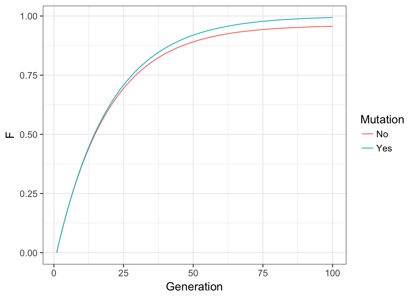
$Expected values for inbreeding F through time for a locus without mutation and one with mutation at a rate of $\mu=0.001$.$

Figure 10.4: Expected values for inbreeding F through time for a locus without mutation and one with mutation at a rate of $\mu=0.001$.

In these data, the overall effect on inbreeding is to modulate autozygosity through time by removing alleles that are identical by descent in the previous generation. The functional consequence here are that while mutation can influence inbreeding to a large degree, it does so with a relatively small impact. If you look back at the changes in allele frequency due to drift, the potential for changing allele frequencies was much greater than we see here. After 100 generations in the code above, even with a $N_e = 10$, there is only a net difference in allele frequencies of $\delta p = 0.0372$! Overall, mutation is the ultimate source of diversity, though has a small (though perceptible) per-generation influence on inbreeding.

As was the case in other situations, there is an expectation for equilibrium with respect to inbreeding based upon both effective population size ($N_e$) and mutation rate ($\mu$). If we set $F_{t+1} = F_t$ and solve, we find the equilibrium inbreeding level to be:

\[ \begin{aligned} \hat{F} &= \frac{1-2\mu}{4N_e\mu + 1 - 2\mu} \\ &\approx \frac{1}{4N_e\mu+1} \end{aligned} \]

with the approximation for small values of $\mu$ (small, as in what we usually see in our data).

10.3 Estimating Mutation

Mutation rates can be estimated from several kinds of data. Here are some simple examples using phenotype and genotype. The end result here is to use observation to uncover an estimate of the rate of mutation, $\mu$, from either or samples or our genetic data.

10.3.1 Phenotypes

Outside some biochemical changes observed in model systems, there are few traits that we can examine directly that are the result of a single mutation event at a single location. While we provide a lot of verbiage to single-gene traits in undergraduate curriculum when introducing Mendelian genetics, there are very few traits that actually respond in that fashion.

The mutation must have a distinctive phenotype. To identify the presence of a mutation, you must have the ability to clearly, and without error, cleanly identify when a mutation arises. This trait must be distinctive in that it has to have a categorical condition. Quantitative traits cannot be used since the contribution of an individual mutation may be minuscule in the trait value. Moreover, several different mutation events, potentially spread throughout the genome, may contribute to the same incremental change in the observed phenotype.
The trait must be fully expressed. Epistatic effects that mask mutants prevent accurate estimation of mutation rates. For example, in the labrador retriever, the locus that controls coat color (brown is recessive to black) can be masked by a second locus that determines if the coat color pigment is put onto the hair shaft (if not the dog is yellow). The presence of this second locus that influences the observed phenotype can prevent the estimation of mutation rates for the first.
The observed phenotype must only be the result of the mutation. If the phenotype is subjected to variation due to environmental effects, this can also cause problems with estimating the mutation rate.

Given these caveats, it is possible to gain mutation estimates from phenotype, it is just difficult in most systems.

As an example, consider the case where a phenotype is governed by the normal dominant/recessive alleles as characterized by Mendel. Mutation rates for the dominant allele can be estimated by examining the number of individuals in the next generation ($x$) that were produced by parents who did not carry the dominant trait (e.g., they were recessive homozygotes). Here the mutation rate is estimated by:

\[ \mu = \frac{x}{2N} \]

Estimation of mutation in recessive alleles can be accomplished in the same way. Here though, offspring are only considered from mating events between individuals known to be homozygous dominant those whose genotype produces the recessive trait. The offspring whose phenotype is recessive ($x$) are those that the dominant allele given by one parent had mutated. As such, since only one parent is contributing, the mutation rate here is estimated as:

\[ \mu = \frac{x}{N} \]

10.3.2 Genotypes

Looking at the genotypes directly can also provide an estimate of mutation rate. I’ll give two quick examples below, as both are relatively straight forward in their implementation. First, if one can maintain lineages of individuals across generations, it becomes relatively easy to monitor the rate at which novel mutations occur. Perhaps the most elegant examples of this approach is that from Lynch et al. (2008) who propagated parallel yeast cell lines across roughly 4,800 divisions. Subsequent sequencing of original and progenitor samples provided an estimated rate of $\mu=0.00000000033$ per generation (much smaller than we have been playing with in this section). They also examined differences in transition and transversion mutations as well as those in the mitochondria. This paper is a tour-de-force and should be read by everyone interested in mutations.

Not everyones study organism fits into a 4000 generation propagation program! That said, there have been some pretty good estimates of mutation rate based upon reconstruction of relatedness among historically separated lineages. If you have a good reconstruction of genetic divergence (as in a phylogeny) and events that have been verified to have specific dates ascribed to them (such as fossil records), you can also estimate mutation rates from these. By far, mtDNA has been used as it has is assumed to be ‘clock-like’ (though see Galtier et al. 2009), though other targets have been used as well. At present, we have several lines of evidence suggesting rates of mutation in various taxonomic groups, each of which may differ substantially. Since rates differ across groups and across regions in the genome, it is important that you consider the consequences that particular values of $\mu$ have on your biological inferences. It is much more common to need an estimate of mutation as an input to another analysis, such as a coalescent model, than to need to estimate it directly from your data. In these common situations, it is good practice for you examine the consequences variation in $\mu$ have on your downstream biological inferences—in some situations a magnitude or more change in mutation may have no appreciable effect whereas in others it may.

Mutant Allele	Frequency
0	\((1-\mu)^2\)
1	\(2\mu(1-\mu)\)
2	\(\mu^2\)