19 Rarefaction

The primary reason for looking at diversity is to perform some comparison, which provides some insights into the biological and/or demographic processes influencing your data. Without a basis for comparison, diversity estimates are just numbers. However, deriving an estimate of diversity is a statistical sampling process and as such we must be aware of the consequences our sampling regime has on the interpretation of the data. This is where rarefaction comes in, a technique commonly used in ecology when comparing species richness among groups.

Here is an example of the problem sampling may interject into your analyses. Consider a single locus with four alleles.

library(gstudio)
data(arapat)
f <- data.frame( Allele=LETTERS[1:4], Frequency=0.25)
f

##   Allele Frequency
## 1      A      0.25
## 2      B      0.25
## 3      C      0.25
## 4      D      0.25

Selected as a random sample from an infinite population. The first sample has 5 individuals.

pop1 <- make_population( f,N=5)
ae1 <- genetic_diversity( pop1, mode="Ae" )
ae1

##   Locus       Ae
## 1 Locus 3.846154

And the second one has 100 individuals.

pop2 <- make_population( f, N=100 )
ae2 <- genetic_diversity( pop2 )
ae2

##   Locus       Ae
## 1 Locus 3.997601

The difference in estimated diversity among these groups are abs( ae1 - ae2 ) = 0.15. Is this statistically different or are they the same? Is it just because we sampled more individuals in the second set that we get higher values of \(A_e\)? Consider the MP20 locus in the beetle data set, it has a total of 19 alleles present. If we subsample this data and estimate the number of observed alleles, we see that there is an asymptotic relationship between sampling effort and estimates of allelic diversity. Here is the code for estimating frequency independent diversity, \(A\), using these data.

loci <- arapat$MP20
sz <- c(2,5,10,15,20,50,100)
sample_sizes <- rep( sz, each=20 )
Ae <- rep(NA,length(sample_sizes))
for( i in 1:length(Ae)){
  loci <- sample( loci, size=length(loci), replace=FALSE)
  Ae[i] <- genetic_diversity( loci[1:sample_sizes[i]], mode="A" )
}

The ‘curvy’ nature of this relationship shows a few things.

It takes a moderate sample size to capture the main set of alleles in the data set. If we are looking at allocating sampling using only 5 individuals per locale, then we are not going to get the majority of the alleles present.

For the rare alleles, you really need to grab large at-site samples if estimates of diversity are the main component of what you are doing. Do rare alleles aid in uncovering the biological processes you are interested in studying? They may or may not.

For most purposes, we will use all the samples we have collected. In many cases though, some locales may not have as many samples as other ones. So, even with these data, if I have one locale with 10 samples and another with 50, how can I determine if the differences observed are due to true differences in the underlying diversity and which are from my sampling? Just as in testing for HWE, we can use our new friend permutation to address the differences.

Rarefaction is the process of subsampling a larger dataset in smaller chunks such that we can estimate diversity among groups using the same number of individuals. Here is an example in the beetle dataset where I am going to look at differences in diversity among samples (\(N = 75\)) collected in the cape regions of Baja California

ae.cape <- genetic_diversity( arapat[ arapat$Species=="Cape", "WNT"] )
ae.cape

##   Locus       Ae
## 1 Locus 1.305052

and compare those to the genetic diversity observed from a smaller collection of individuals sampled from mainland Mexico (\(N=36\)).

ae.mainland <- genetic_diversity( arapat[ arapat$Species=="Mainland", "WNT"] )
ae.mainland

##   Locus       Ae
## 1 Locus 1.033889

The observed difference in effective allelic diversity, \(A_{e,mainland} == A_{e,cape}\), could be because the Cape region of Baja California is more diverse or it could be because there are twice as many individuals in that sample.

To perform a rarefaction on these data, we do the following:

Use the size of the smallest population (\(N\)) as the sample size for all estimates. Randomly sample individuals, without replacement, from the larger dataset in allocations of size \(N\).

Estimate diversity parameters on these subsamples and repeat to create a ‘null distribution’ of estimated diversity values.

Compare your observed value in the smallest population to that distribution created by subsampling the larger population.

From the data set, this is done by

cape.pop <- arapat[ arapat$Species=="Cape","WNT"]
null.ae <- rarefaction( cape.pop, mode="Ae",size=36)
mean(null.ae)

## [1] 1.314233

So even if the samples sizes are the same, the mean level of diversity remains relatively constant. The range in diversity

range(null.ae)

## [1] 1.000000 1.829217

is quite large. Since this estimate is frequency based, random samples of alleles change the underlying estimate of Ae during each permutation.

The observed estimate of diversity in the Mainland populations does fall within this range. However, the null hypothesis states that \(A_{e,mainland} = A_{e,cape}\) and if this is true, once we standardize sample size, we can take the distribution of permuted Ae values as a statement about what we should see if the null hypothesis were true. As such, we can treat it probabilistically and estimate the probability that \(A_e\), Mainland is drawn from this distribution.

null.ae <- c( null.ae, ae.mainland[1,1])
P <- sum( ae.mainland <= null.ae ) / ( length(null.ae) )
P

## [1] 0.001

Or graphically, it can be depicted as below.

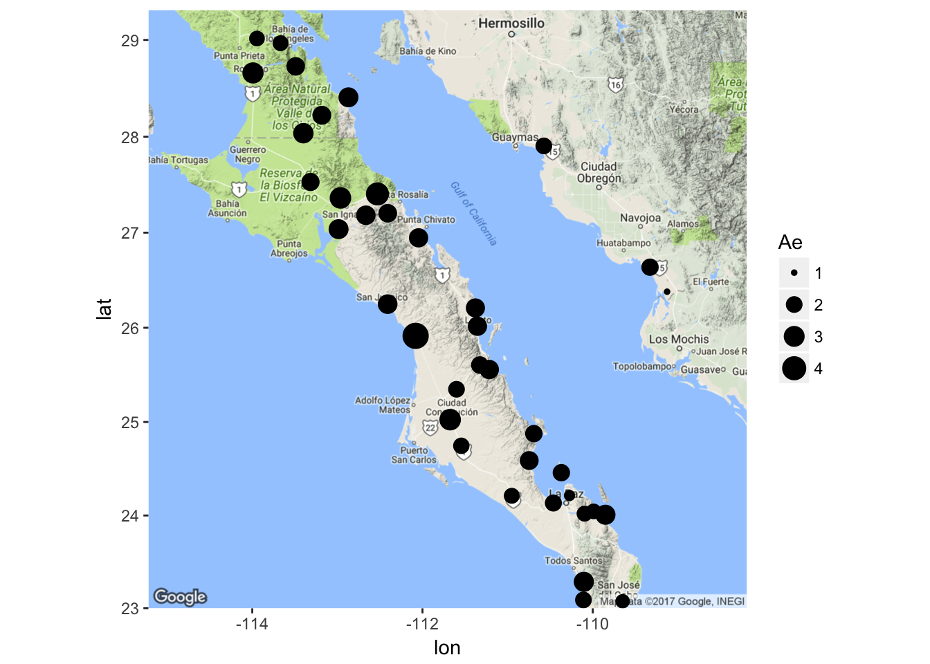
19.1 Mapping Diversity

Estimating diversity is great and being able to compare two or more groups for their levels of diversity is even better. But often we are looking for spatial patterns in our data. Both R and gstudio provide easy interfaces for plotting data and later in the text we will see how to integrate raster and vector data into our workflows for more sublime approaches to characterizing population genetic processes. In the mean time, it is amazingly easy to use basic plotting commands to get pretty informative output. In this example, I extract the mean coordinate of each stratum in the arapat dataset and then estimate diversity at the level of these partitions and merge the diversity estimates for the AML locus into the coordinate data.frame.

library(gstudio)
data(arapat)
diversity <- genetic_diversity(arapat, stratum="Population", mode="Ae")
coords <- strata_coordinates(arapat)
coords <- merge( coords, diversity[ diversity$Locus == "AML", ] )

Then, I grab a map from the Google server and map my populations with diversity depicted as differences in the size of the points. Note that the ggmap() function provides the base map that is retrieved but when we use geom_point() we need to specify the aes() and the data= part as these data are from the data.frame we made, not from the map we grabbed from Google.

library(ggmap)
map <- population_map(coords)
ggmap(map) + geom_point( aes(x=Longitude,y=Latitude,size=Ae), data=coords)