14 Pedigrees

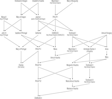
Pedigrees are visual representations of genetic relations. They are extremely important for estimating inbreeding and following traits or diseases in lineages. In this lecture, we will learn:

Symbology used in pedigrees
Estimation of inbreeding F from a given pedigree
Approaches for plotting pedigrees

In the analysis of pedigrees, we often use the following terminology:

Consanguineous mating (lit. “Of the same blood”). The condition where individuals who are related produce offspring.
Biparental Inbreeding (see consanguineous mating).

A pedigree is simply a graphical representation characterizing the relationship amongst ancestral individuals. This tool is very helpful for understanding the process of inbreeding when it occurs during a handful of generations.

Perhaps the most studied pedigree is that of the Hapsburg Dynasty, dating from 1516-1700, which controlled most of what we call modern Europe. Some of the European Royalty were interbred to maintain familial relationships and consolidate power. Examples include:

King	Queen	Consanguineous Marriage
Philip I (1478-1506)	Joanna I of Castile & Aragon	Third cousins
Charles I (1500-1558)	Isabella of Portugal	First cousins
Philip II (1527-1598)	Mary of Portugal	Double first cousins
\(\;\)	Mary I of England	First cousins once removed
\(\;\)	Anna of Austria	Uncle-Niece
Philip III (1578-1621)	Margaret of Austria	First cousins once removed
Philip IV (1605-1665)	Elizabeth of Bourbon	Third cousins
\(\;\)	Mariana of Austria	Uncle-Niece
Charles II (1661-1700)	Marie Louise d’Orleans	Second cousins

Hapsburg Dynasty | Piliip I (\(F=0.025\)) \(\to\) Charles II (\(F=0.254\))

knitr::include_graphics("./media/HapsburgPedigree.png")

A pedigree of the Hapsburg Dynasty. This pattern of mating resulted in individual inbreeding going from \(F=0.025\) for Philip I to \(F=0.254\) for Charles II.

In this lineage, there were two genetic disorders that became paramount:

Pituitary hormone deficiency
Distal renal tubular acidosis

Pedigree Symbology

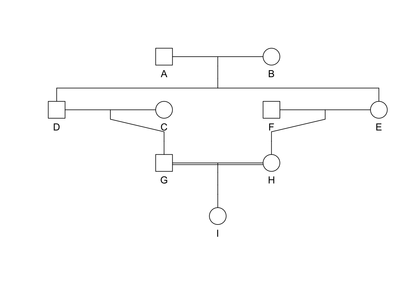
knitr::include_graphics("media/pedigree1.png")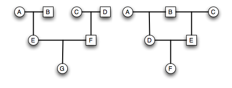

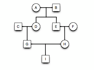
Each row is a generation.
Lines within a generation represent mating events that result in offspring.
Lines between generations represent descent.
Individuals are labeled uniquely.
Sex is indicated by shape (square=male, circle=female, diamond=unknown).
Traits can be mapped onto the pedigree using additional colors & symbols

knitr::include_graphics("./media/pedigree0.png")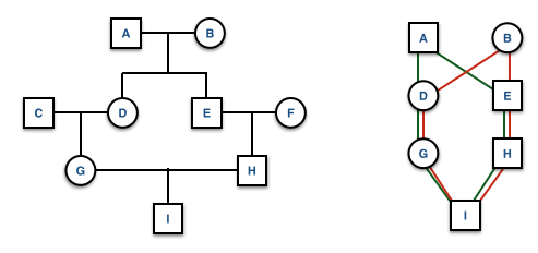

Extraneous individuals may be removed from the depiction. Why is it that C and F are not shown on the pedigree on the right side?

Estimating Inbreeding From Pedigrees

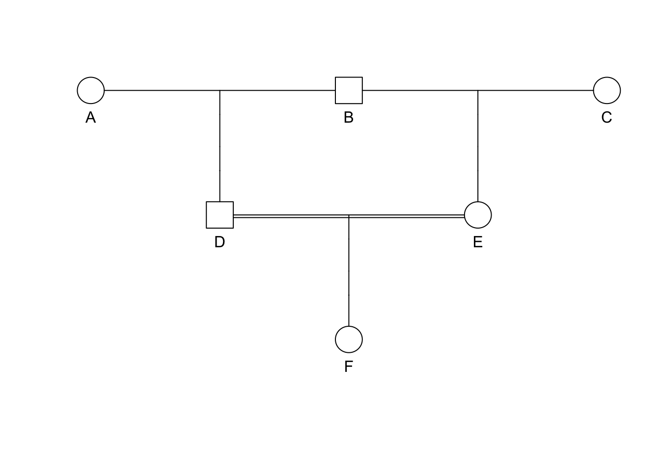
The inbreeding coefficient, F, of an individual is determined by the probability that a pair of alleles carried by gametes are IBD from a recent common ancestor.

knitr::include_graphics("./media/pedigree2.png")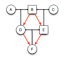

F has same grandfather on both sides.
D and E are half-sibs sharing father B.
B passed one of his alleles, say \(A_1\), to both D and B.
D passed allele \(A_1\) to F and E passed allele \(A_1\) to F, which means
F has some non-zero probability of being autozygous

Expectations for \(F\) in a pedigree.

knitr::include_graphics("./media/pedigree2.png")

Label alleles in B as \(\alpha\) and \(\beta\).
The alleles B gives to D & E are \(\{\alpha, \alpha\}\), \(\{\alpha, \beta\}\), \(\{\beta, \alpha\}\), or \(\{\beta, \beta\}\)
Each potential allele pair occurs at: \(\left(\frac{1}{2}\right)^2 = \frac{1}{4}\)
If B gives \(\{\alpha,\alpha\}\) or \(\{\beta, \beta\}\) then the two alleles in the children of B are autozygous (by definition).
If B gives \(\{\alpha,\beta\}\) or \(\{\beta, \alpha\}\) then the two alleles in the children of B are autozygous only if the alleles \(\alpha\) and \(\beta\) are autozygous.
The probability of \(\alpha\) and \(\beta\) being autozygous in B is given by the inbreeding coefficient \(F\) for B (denoted \(F_B\)).

14.1 Expectations for F in a pedigree.

knitr::include_graphics("./media/pedigree2.png")

Transition probabilities for all cases of alleles within the children of B are:

\(P({\alpha,\alpha}|\mathbf{B}) = \frac{1}{4}\)
\(P({\alpha,\beta}|\mathbf{B}) = \frac{1}{4}F_A\)
\(P({\beta,\alpha}|\mathbf{B}) = \frac{1}{4}F_A\)
\(P({\alpha,\alpha}|\mathbf{B}) = \frac{1}{4}\)

knitr::include_graphics("./media/pedigree2.png")

Total probability for B donating autozygous alleles to his offspring are then:
[ = + F_A + F_A + \ = + F_A \ = (1.0 + F_A) \ ]

Expectations for \(F\) in a pedigree.

knitr::include_graphics("./media/pedigree2.png")

The transition probabilities for the alleles that D & E received from B and passes on to F are \(\frac{1}{2}\) for each.
The total probability that the two alleles in F are autozygous (Identical By Decent; IBD) is:
[ F = (1.0 + F_A) \ = ( )^3 (1.0 + F_A) ]

Generalized Formula for Inbreeding | Chain Counting Method

knitr::include_graphics("./media/pedigree2.png")

[ F = ( )^i (1.0 + F_A) ] where the exponent \(i\) is the length of the ancestral loop (e.g., the number of steps starting at F and going trough the common ancestor and back to F) which in this case is DBE (the common ancestor is underlined).

Several Ancestral Loops

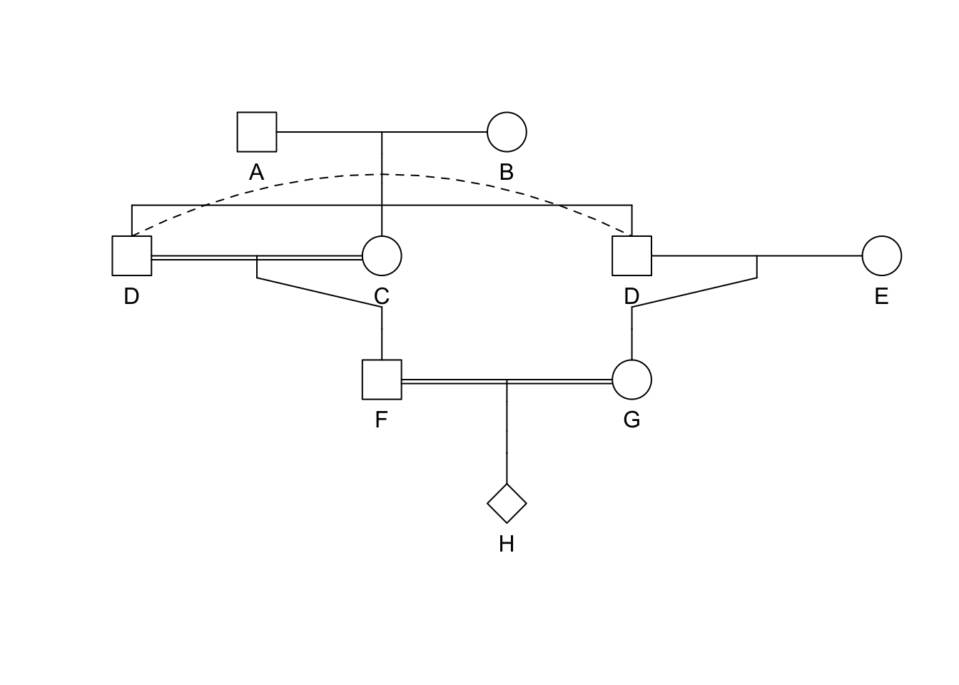
knitr::include_graphics("./media/pedigree4.png")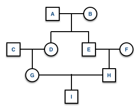

If there is more than one ancestral loop, then the final inbreeding coefficient, F, is the sum of the F estimated across each loop (assuming there are \(K\) different loops in the pedigree). In this example you would use both GDAEH and GDBEH.
[ F = _{k=1}^{K} ]

N.B. Each ancestor may have different \(F_k\) values.

Strategies for Pedigrees

Here is a basic strategy for solving pedigree questions.

Draw the pedigree
Identify common ancestor(s)
Trace ancestral loop(s)
Annotate all ancestral loops indicating the common ancestor
The length of each ancestral loop is \(i\)
Plug into the equation for inbreeding statistic F for each loop.
Final F is sum of all estimated F from each loop.

Easy Example, F=?

library(kinship2)
id    <- LETTERS[1:6]
dadid <- c(NA,NA,NA,"B","B","D")
momid <- c(NA,NA,NA,"A","C","E")
sex   <- c("female","male","female","male","female","female")
ped <- pedigree( id, dadid, momid, sex)
ped

Pedigree object with 6 subjects
Bit size= 3

plot(ped)

Ancestral loop: DBE,
\(i = 3\),
\(F_F = \left( \frac{1}{2} \right)^3(1+F_A)\).

Easy Example, F=?

library(kinship2)
id    <- LETTERS[1:9]
momid <- c(NA,NA,NA,"B","B",NA,"C","E","H")
dadid <- c(NA,NA,NA,"A","A",NA,"D","F","G")
sex   <- c("male","female","female","male","female","male","male","female","female")
ped <- pedigree( id, dadid, momid, sex)
plot(ped)

Ancestral loop: GDAEH, GDBEH, \(F_I = \left[ \left( \frac{1}{2} \right)^5(1+F_A) \right] + \left[ \left( \frac{1}{2} \right)^5(1+F_B) \right]\).

Medium Example, F=?

id    <- LETTERS[1:8]
dadid <- c(NA,NA,"A","A",NA,"D","D","F")
momid <- c(NA,NA,"B","B",NA,"C","E","G")
sex   <- c("male","female","female","male","female","male","female","unknown")
ped <- pedigree( id, dadid, momid, sex)
suppressWarnings(plot(ped))

Ancestral loop: GDAEH, GDBEH, \(F_I = \left[ \left( \frac{1}{2} \right)^5(1+F_A) \right] + \left[ \left( \frac{1}{2} \right)^5(1+F_B) \right]\).

14.2 Drawing Pedigrees

Example Pedigree

library(kinship2)
id    <- LETTERS[1:5]
dadid <- c(NA,NA,"A","A","A")
momid <- c(NA,NA,"B","B","B")
sex   <- c("male","female","male","female","female")
data <- data.frame( id, dadid,momid,sex)
data

  id dadid momid    sex
1  A  <NA>  <NA>   male
2  B  <NA>  <NA> female
3  C     A     B   male
4  D     A     B female
5  E     A     B female

Example Pedigree

ped <- pedigree(data$id, data$dadid, data$momid, data$sex)
ped

Pedigree object with 5 subjects
Bit size= 4

summary(ped)

       Length Class  Mode     
id     5      -none- character
findex 5      -none- numeric  
mindex 5      -none- numeric  
sex    5      factor numeric

Example Pedigree

plot.pedigree(ped)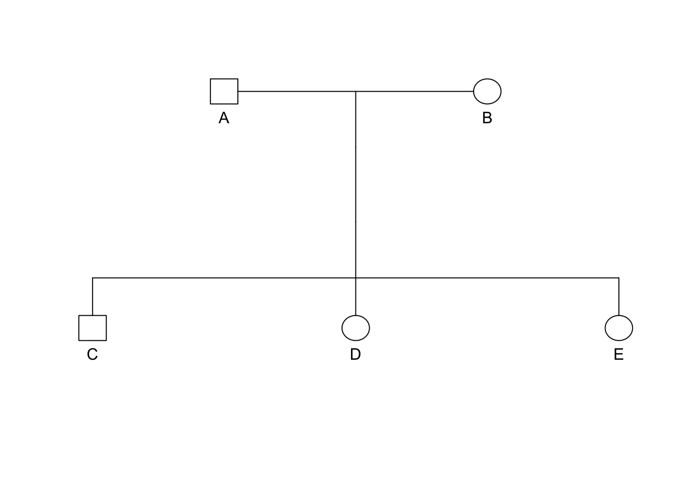

Decay of \(F\), The effects of size in the ancestral loop

library(ggplot2)
df <- data.frame( i=seq(4,20,by=2) )
df$F <- 0.5^df$i
ggplot( df, aes(x=i,y=F) ) + geom_line(color="red")

14.3 Skills

This lecture covered the creation and analysis of pedigree data. At the end of this lecture you should be able to:

first skill
second skill

id    <- LETTERS[1:9]
momid <- c(NA,NA,NA,"B","B",NA,"C","E","H")
dadid <- c(NA,NA,NA,"A","A",NA,"D","F","G")
sex   <- c("male","female","female","male","female","male","male","female","female")
brown_eyes <- c(1,0,0,1,1,NA,1,1,0)
college <- c(0,1,0,0,0,0,1,1,1)
likes_asparagus <- c(0,1,0,0,1,1,0,1,1)
traits <- cbind( brown_eyes, college, likes_asparagus)

ped <- pedigree( id, dadid, momid, sex, affected = traits)
plot(ped)
pedigree.legend( ped, location="bottomleft",radius=.2)

library(gstudio)
p1 <- c("Ai","Aj")
p2 <- c("Ak","Al")
offs <- c(  locus( c(p1[1],p2[1]) ), 
            locus( c(p1[2],p2[1]) ), 
            locus( c(p1[1],p2[2]) ),
            locus( c(p1[2],p2[2]) ) )
offs

[1] "Ai:Ak" "Aj:Ak" "Ai:Al" "Aj:Al"

Relationship	\(k_0\)	\(k_1\)	\(k_2\)	\(r\)
Identical Twins	0	0	1	1
Full Sibs	0.25	0.5	0.25	0.5
Parent Offspring	0	1	0	0.5
Half Sib	0.5	0.5	0	0.25
Aunt-nephew	0.5	0.5	0	0.25
First Cousin	0.75	0.25	0	0.125
Unrelated	1	0	0	0

sdf

ped <- pedigree( id, dadid, momid, sex, affected = traits)
plot(ped)
pedigree.legend( ped, location="bottomleft",radius=.2)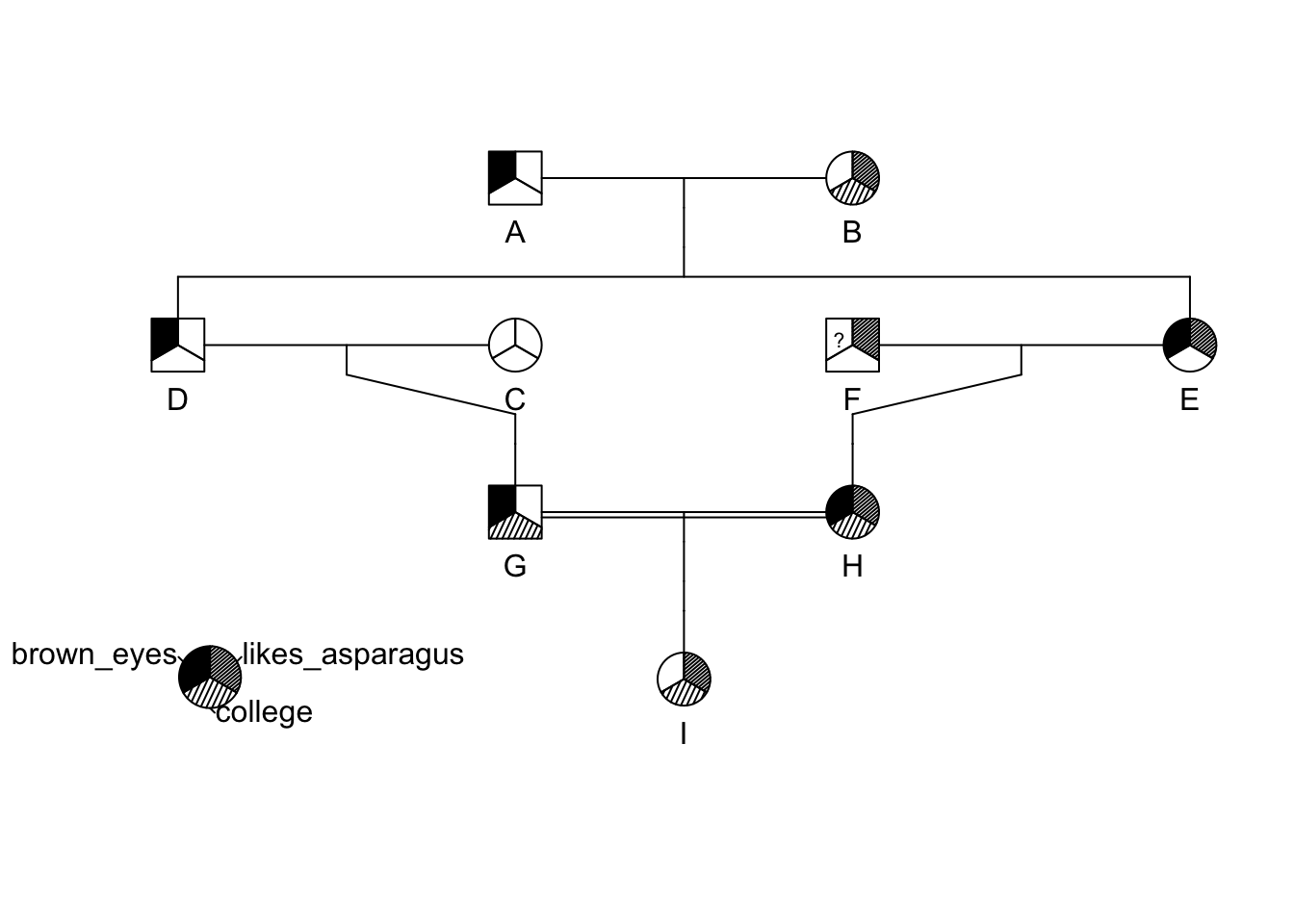

kinship(ped)

      A     B     C      D      E     F       G       H       I
A 0.500 0.000 0.000 0.2500 0.2500 0.000 0.12500 0.12500 0.12500
B 0.000 0.500 0.000 0.2500 0.2500 0.000 0.12500 0.12500 0.12500
C 0.000 0.000 0.500 0.0000 0.0000 0.000 0.25000 0.00000 0.12500
D 0.250 0.250 0.000 0.5000 0.2500 0.000 0.25000 0.12500 0.18750
E 0.250 0.250 0.000 0.2500 0.5000 0.000 0.12500 0.25000 0.18750
F 0.000 0.000 0.000 0.0000 0.0000 0.500 0.00000 0.25000 0.12500
G 0.125 0.125 0.250 0.2500 0.1250 0.000 0.50000 0.06250 0.28125
H 0.125 0.125 0.000 0.1250 0.2500 0.250 0.06250 0.50000 0.28125
I 0.125 0.125 0.125 0.1875 0.1875 0.125 0.28125 0.28125 0.53125