11 Selfing

Inbreeding is one of the most common deviations from random mating (and hence Hardy-Weinberg Equilibrium) that we encounter in natural populations. Inbreeding is defined, sensu stricto, as mating between two related individuals. This ranges from complete selfing, where one parent alone produces offspring, to consanguineous mating, where individuals with some degree of relatedness produce offspring. The genetic consequences of inbreeding are entirely in how alleles are arranged into genotypes, not in changing allele frequencies.

The primary consequence of inbreeding is a reduction in the frequency of the heterozygous genotype. Consider the following Punnet square where a heterozygote is producing a selfed offspring.

	$A$	$B$
$A$	$AA$	$AB$
$B$	$AB$	$BB$

The offspring in the next generation are only 50% heterozygotes. Each generation of selfing, homozygotes produce homozygotes but only half of the offspring from heterozygotes stay as such. This process increases the relative frequency of homozygous genotypes in the population, though if you look at the offspring, the frequency of alleles do not change—there are as many A alleles as B alleles in the next generation of selfing.

Conceptually, we can define an inbreeding parameter, $F$, depicting the extent to which genotype frequencies have deviated from HWE due to inbreeding. But to do so, we need to differentiate between homozygote genotypes that have the same alleles because they are inbred (e.g., both alleles can be traced to a single allele in common ancestor) from those that are identical because they just happen to have the same allele (not of common ancestry). For this, we will define terms for these genotypes as:

Autozygous - Two alleles that are identical within a genotype because they came from the same individual in the previous generation. These alleles are Identical by Descent and will be found in the population at a rate of $pF$.

Allozygous - Two alleles that are identical within a genotype but they came from alternate individuals in the parental generation. These alleles have Identity by State and are expected to occur at a frequency of $p^2(1-F)$.

Together, the expected frequency of the AA genotype, $E[AA] = p^2(1-F) + pF$.

At the extremes, if there is no inbreeding—all homozygotes are allozygous—the inbreeding statistic, $F=0$ and the expectation reduces to $E[AA] = p^2$. Conversely, if all offspring are the result of selfing, $F=1$ and $E[AA] = p$.

Often the parameter $F$ is the subject of our analyses and the item that is to be estimated from genetic data. Give the definition above, $F$ is defined as the proportional loss of heterozygosity and is estimated as:

\[ \begin{aligned} F &= \frac{H_e - H_o}{H_e} \\ &= 1 - \frac{H_o}{H_e} \end{aligned} \]

The key point here is that inbreeding (autozygosity) is estimated ‘relative’ to the expected frequencies of non-inbred heterozygotes (allozygosity).

Selfing is the most extreme form of inbreeding is that of selfing—one parent donates both gametes to the offspring. In selfing systems, the frequency of genotypes $P = freq(AA)$, $Q = freq(AB)$, and $R = freq(BB)$, change in through time in a predictable fashion providing us a quantitative approach to characterizing the duration of inbreeding from allele and genotype frequencies.

From first principles, selfing for these genotypes produces the following expected offspring genotype frequencies:

Parent	Offspring	Frequency
$AA$	$AA$	$P$
$AB$	$1/4\;AA$	$Q/4$
	$1/2\;AB$	$Q/2$
	$1/4\;BB$	$Q/4$
$BB$	$BB$	$R$

Such that the genotype frequencies in the next generation are:

\[ \begin{aligned} P_{t+1} &= P_t + \frac{1}{4}Q_t \\ Q_{t+1} &= \frac{1}{2}Q_t \\ R_{t+1} &= R_t + \frac{1}{4}R_t \end{aligned} \]

The interesting thing here is that the allele frequencies at the next generation are derived from the genotype frequencies as:

\[ p_{t+1} = P_{t+1} + \frac{1}{2}Q_{t+1} \]

But with a little re-arrangement of terms, we see that

\[ \begin{aligned} p_{t+1} &= P_{t+1} + \frac{1}{2}Q_{t+1} \\ &= \left(P_t + \frac{1}{4}Q_t \right) + \frac{1}{2}\left( \frac{1}{2}Q_t \right) \\ &= P_t + \frac{1}{2}Q_t \\ &= p_t \end{aligned} \]

showing that while genotype frequencies change with each generation of inbreeding, the underlying allele frequencies remain constant! Inbreeding only changes how alleles are packed into genotypes and in not changing frequencies, does not result in evolutionary change, sensu stricto.

11.1 Changes in F

For every generation with selfing, the average level of inbreeding in the population will increase. The amount it increases depends upon how inbred the population already is, outbred populations will have larger $\delta F$ than similar populations with higher initial $F$.

11.1.1 Theoretical Expectations

As expected, selfing changes the estimate of $F$ as well. It changes across generations with continued selfing as:

\[ F_1 = 1 - \frac{H_O}{H_E} = 1 - \frac{Q_1}{2pq} \]

for the first generation,

\[ F_2 = 1 - \frac{ \frac{Q_1}{2} }{2pq} \]

for the second,

\[ F_3 = \frac{\frac{Q_2}{2}}{2pq} = \frac{\frac{\frac{Q_1}{2}}{2}}{2pq} \]

and the next

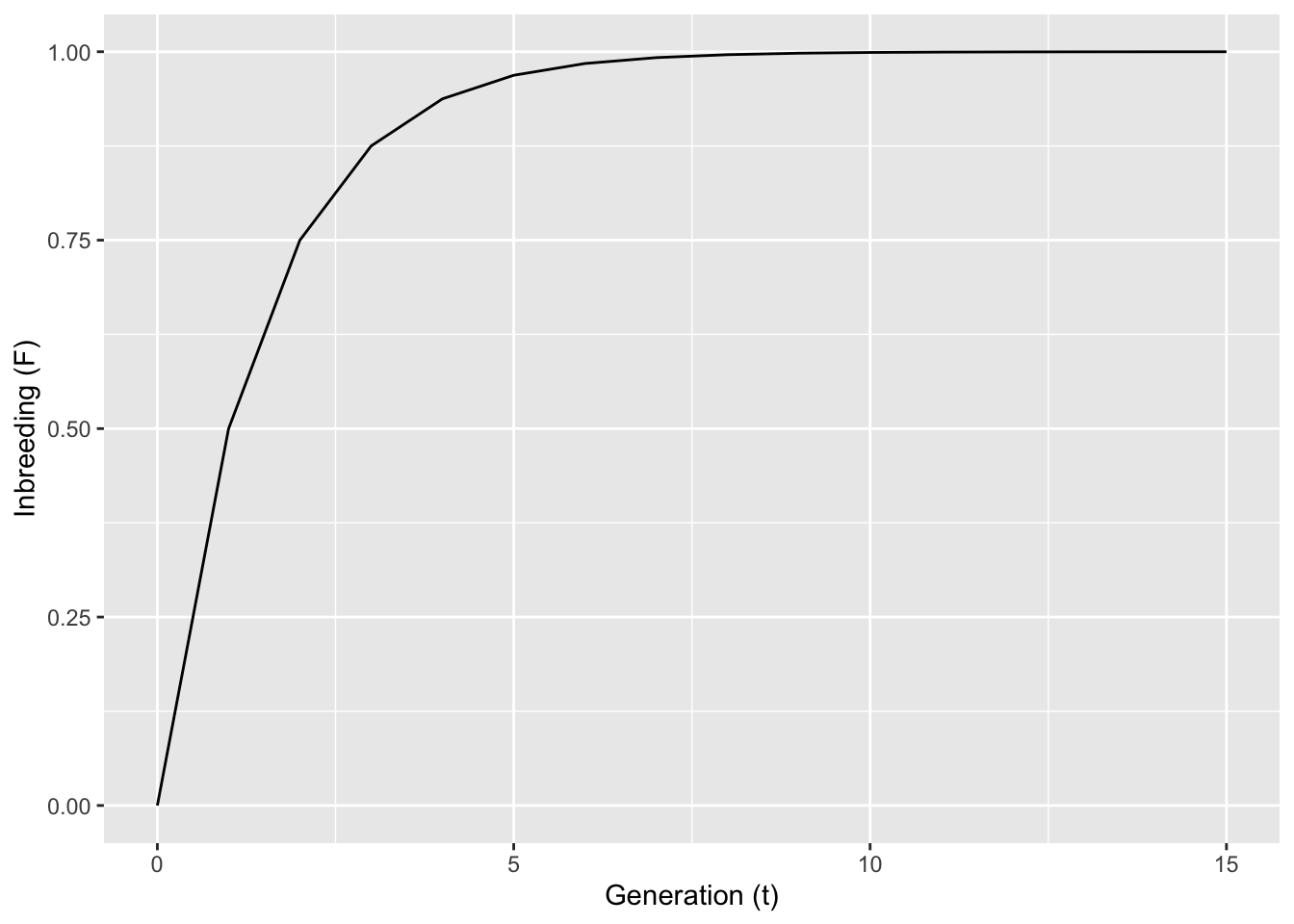
\[ F_4 = \frac{\frac{Q_3}{2}}{2pq} = \frac{\frac{\frac{Q_2}{2}}{2}}{2pq} = \frac{\frac{\frac{\frac{Q_1}{2}}{2}}{2}}{2pq} \]

and so on. Numerically, if $F_1=0$, then $F2 = 0.50, F3 = 0.75, and F4 = 0.875. Each generation, $F$ approaches 1.0 by half way. From this pattern, the change in $F$ each generation can be estimated as:

\[ F_{t+1} = \frac{1}{2} + \frac{1}{2}F_t \]

for each generation or

\[ F_t = 1 - \left(\frac{1}{2}\right)^t(1-F_O) \]

for any arbitrary time, $t$, in the future given some starting level of inbreeding. This expectation looks like:

library(ggplot2)
T <- 0:15
F <- 1 - 0.5^T
df <- data.frame( T, F)
ggplot(df,aes(T,F)) + geom_line() + xlab("Generation (t)") + ylab("Inbreeding (F)")

11.2 Simulation Example

These smooth expectations are nice but real data is a bit more complex. Real data is not so clean but it is pretty easy to simulate this process and measure the change in inbreeding through time. Here is how that can be done.

First, I’m going to start with a population in HWE with allele frequencies of $p=q$. To do this, we start by importing the gstudio library and making raw genotypes. We can replicate them to make a starting population with $N=100$ individuals.

library(gstudio)
AA <- locus( c("A","A") )
AB <- locus( c("A","B") )
BB <- locus( c("B","B") )
pop <- data.frame(ID=1:100, Locus1=c( rep(AA,25), rep(AB,50), rep(BB,25) ) )

Just to check, we can see the starting allele frequencies as:

frequencies(pop)

##    Locus Allele Frequency
## 1 Locus1      A       0.5
## 2 Locus1      B       0.5

The inbreeding parameter, $F$, is estimated on a data.frame object that has at least one column of data of type locus using the wrapper function genetic_diversity() and passing it the mode="Fis" option—the ‘is’ subscript here is because there are additional $F$ statistics that may be calculated for different groups of individuals which will be covered in the section on genetic structure. The parameter $F$ is estimated for each locus and the results are given in a data.frame.

genetic_diversity(pop,mode="Fis")

##    Locus Fis
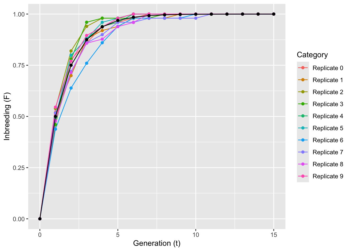
## 1 Locus1   0

I am going to simulate 10 replicate runs of selfing, each starting with this very population. During each replicate, each individual will produce one and only one offspring through selfing using the function mate() and iterated across generations as in the expectation. The parameter F will be recorded after all replications are finished plot against time.

df$Category = "Expectations"
for( rep in 0:9 ) {
  data <- pop
  F <- rep(0, length(T) )
  for(t in T){
    # estimate F
    F[(t+1)] <- genetic_diversity(data,mode="Fis")$Fis[1]
    # self all adults to make offspring
    data <- mate( data, data, N=1 )
  }
  df.rep <- data.frame( T, F, Category=paste("Replicate",rep))
  df <- rbind( df, df.rep )
}

The variance around expectation is moderate shows that even if all expectations are met, real data is a bit messy—perhaps expectations are more of what you’d call ‘guidelines’ than strict rules.

Figure 11.1: Replicate simulations of inbreeding in purely selfing populations (colored lines) with theoretical expectation (black line).

	\(A\)	\(B\)
\(A\)	\(AA\)	\(AB\)
\(B\)	\(AB\)	\(BB\)

Parent	Offspring	Frequency
\(AA\)	\(AA\)	\(P\)
\(AB\)	\(1/4\;AA\)	\(Q/4\)
	\(1/2\;AB\)	\(Q/2\)
	\(1/4\;BB\)	\(Q/4\)
\(BB\)	\(BB\)	\(R\)