4 Allele Frequencies & HWE

This chapter covers estimating allele and genotype frequencies, testing for Hardy-Weinberg Equilibrium, and rarefaction analysis.

library(gstudio)
library(dplyr)
library(ggplot2)
data(arapat)

4.1 Allele Frequencies

The frequencies() function is an S3 generic that works on both individual locus vectors and entire data.frames.

4.1.1 Single Locus

arapat |>
  pull(LTRS) |>
  frequencies()

  Allele Frequency
1     01  0.523416
2     02  0.476584

4.1.2 Entire Data Frame

When applied to a data.frame, frequencies() returns frequencies for all locus columns:

freqs <- arapat |>
  frequencies()

freqs |>
  head(12)

   Locus Allele   Frequency
17   AML     01 0.001470588
18   AML     02 0.001470588
19   AML     03 0.019117647
20   AML     04 0.126470588
21   AML     05 0.070588235
22   AML     06 0.072058824
23   AML     07 0.235294118
24   AML     08 0.255882353
25   AML     09 0.145588235
26   AML     10 0.014705882
27   AML     11 0.039705882
28   AML     12 0.016176471

4.1.3 By Stratum

Add a stratum argument to partition frequencies by population:

freqs_pop <- arapat |>
  frequencies(stratum = "Species")

freqs_pop |>
  head(12)

   Stratum Locus Allele Frequency
1     Cape   AML     01 0.0000000
2     Cape   AML     02 0.0000000
3     Cape   AML     03 0.0915493
4     Cape   AML     04 0.6056338
5     Cape   AML     05 0.3028169
6     Cape   AML     06 0.0000000
7     Cape   AML     07 0.0000000
8     Cape   AML     08 0.0000000
9     Cape   AML     09 0.0000000
10    Cape   AML     10 0.0000000
11    Cape   AML     11 0.0000000
12    Cape   AML     12 0.0000000

Because the result is a tidy data frame, dplyr summaries follow directly, for example the most common allele at each locus in each species:

freqs_pop |>
  group_by(Stratum, Locus) |>
  slice_max(Frequency, n = 1, with_ties = FALSE) |>
  filter(Locus %in% c("LTRS", "WNT"))

# A tibble: 6 × 4
# Groups:   Stratum, Locus [6]
  Stratum   Locus Allele Frequency
  <chr>     <chr> <chr>      <dbl>
1 Cape      LTRS  02         0.92 
2 Cape      WNT   02         0.865
3 Mainland  LTRS  02         0.736
4 Mainland  WNT   01         0.983
5 Peninsula LTRS  01         0.692
6 Peninsula WNT   03         0.609

4.1.4 Selecting Specific Loci

arapat |>
  frequencies(loci = c("LTRS", "WNT"))

  Locus Allele   Frequency
1  LTRS     01 0.523415978
2  LTRS     02 0.476584022
3   WNT     01 0.357954545
4   WNT     02 0.181818182
5   WNT     03 0.430397727
6   WNT     04 0.026988636
7   WNT     05 0.002840909

4.2 Frequency Matrix

The frequency_matrix() function produces a wide-format matrix of allele frequencies:

fm <- arapat |>
  frequency_matrix(stratum = "Species")

fm[, 1:8]

    Stratum      AML-01      AML-02    AML-03    AML-04     AML-05     AML-06
1      Cape 0.000000000 0.000000000 0.0915493 0.6056338 0.30281690 0.00000000
2  Mainland 0.000000000 0.000000000 0.0000000 0.0000000 0.00000000 0.00000000
3 Peninsula 0.002016129 0.002016129 0.0000000 0.0000000 0.01008065 0.09879032
     AML-07
1 0.0000000
2 0.0000000
3 0.3225806

4.3 Genotype Counts and Frequencies

4.3.1 Genotype Counts per Stratum

The genotype_counts() function summarizes non-missing genotype counts per locus, optionally by stratum:

arapat |>
  genotype_counts()

    Stratum   N LTRS WNT  EN  EF ZMP AML ATPS MP20
ALL     ALL 363  363 352 360 361 330 340  363  358

arapat |>
  genotype_counts(stratum = "Species")

            Stratum   N LTRS WNT  EN  EF ZMP AML ATPS MP20
Cape           Cape  75   75  74  75  75  70  71   75   75
Mainland   Mainland  36   36  30  35  34  20  21   36   33
Peninsula Peninsula 252  252 248 250 252 240 248  252  250

4.3.2 Genotype Frequencies

The genotype_frequencies() function returns observed and expected genotype counts for a locus vector:

arapat |>
  pull(LTRS) |>
  genotype_frequencies()

  Genotype Observed  Expected
1    01:01      147  99.44904
2    01:02       86 181.10193
3    02:02      130  82.44904

4.4 Hardy-Weinberg Equilibrium

The hwe() function tests for HWE using a chi-square approximation:

arapat |>
  filter(Species == "Mainland") |>
  hwe()

Warning in genotype_frequencies(x[[locus]]): Some genotype expectations are <
5, a continuity correction should be applied.  See ?hwe

Warning in hwe(filter(arapat, Species == "Mainland")): Under 50 samples for
LTRS this may not be a good approximation.

Warning in hwe(filter(arapat, Species == "Mainland")): Fewer than 5 genotypes
expected at LTRS consider collapsing alleles.

Warning in genotype_frequencies(x[[locus]]): Some genotype expectations are <
5, a continuity correction should be applied.  See ?hwe

Warning in hwe(filter(arapat, Species == "Mainland")): Under 50 samples for WNT
this may not be a good approximation.

Warning in hwe(filter(arapat, Species == "Mainland")): Fewer than 5 genotypes
expected at WNT consider collapsing alleles.

Warning in genotype_frequencies(x[[locus]]): Some genotype expectations are <
5, a continuity correction should be applied.  See ?hwe

Warning in hwe(filter(arapat, Species == "Mainland")): Under 50 samples for EN
this may not be a good approximation.

Warning in hwe(filter(arapat, Species == "Mainland")): Fewer than 5 genotypes
expected at EN consider collapsing alleles.

Warning in genotype_frequencies(x[[locus]]): Some genotype expectations are <
5, a continuity correction should be applied.  See ?hwe

Warning in hwe(filter(arapat, Species == "Mainland")): Under 50 samples for EF
this may not be a good approximation.

Warning in hwe(filter(arapat, Species == "Mainland")): Fewer than 5 genotypes
expected at EF consider collapsing alleles.

Warning in genotype_frequencies(x[[locus]]): Some genotype expectations are <
5, a continuity correction should be applied.  See ?hwe

Warning in hwe(filter(arapat, Species == "Mainland")): Under 50 samples for ZMP
this may not be a good approximation.

Warning in hwe(filter(arapat, Species == "Mainland")): Fewer than 5 genotypes
expected at ZMP consider collapsing alleles.

Warning in genotype_frequencies(x[[locus]]): Some genotype expectations are <
5, a continuity correction should be applied.  See ?hwe

Warning in hwe(filter(arapat, Species == "Mainland")): Under 50 samples for AML
this may not be a good approximation.

Warning in hwe(filter(arapat, Species == "Mainland")): Fewer than 5 genotypes
expected at AML consider collapsing alleles.

Warning in genotype_frequencies(x[[locus]]): Some genotype expectations are <
5, a continuity correction should be applied.  See ?hwe

Warning in hwe(filter(arapat, Species == "Mainland")): Under 50 samples for
ATPS this may not be a good approximation.

Warning in hwe(filter(arapat, Species == "Mainland")): Fewer than 5 genotypes
expected at ATPS consider collapsing alleles.

Warning in genotype_frequencies(x[[locus]]): Some genotype expectations are <
5, a continuity correction should be applied.  See ?hwe

Warning in hwe(filter(arapat, Species == "Mainland")): Under 50 samples for
MP20 this may not be a good approximation.

Warning in hwe(filter(arapat, Species == "Mainland")): Fewer than 5 genotypes
expected at MP20 consider collapsing alleles.

  Locus   statistic df      p.value
1  LTRS   0.9082806  1 3.405710e-01
2   WNT  29.2542373  1 6.347726e-08
3    EN  19.7817078  3 1.883729e-04
4    EF   0.3545808  1 5.515314e-01
5   ZMP   5.0927978  1 2.402540e-02
6   AML  36.8802692  6 1.858093e-06
7  ATPS  43.9698647  6 7.494505e-08
8  MP20 161.5565210 45 4.773959e-15

The output includes the chi-square statistic, degrees of freedom, and p-value for each locus. Significant p-values indicate departures from HWE expectations.

4.4.1 Interpreting Results

Departures from HWE can arise from:

Non-random mating (inbreeding, assortative mating)
Population substructure (Wahlund effect)
Selection at or near the marker locus
Small population size (genetic drift)

4.5 Rarefaction

The rarefaction() function subsamples the data repeatedly at a smaller sample size to estimate the distribution of a diversity statistic:

rare_vals <- arapat |>
  pull(LTRS) |>
  rarefaction(mode = "Ae", size = 20, nperm = 199)

data.frame(Ae = rare_vals) |>
  ggplot(aes(Ae)) +
  geom_histogram(bins = 20, fill = "steelblue") +
  labs(title = "Rarefied Ae at LTRS", x = "Effective alleles", y = "Count") +
  theme_minimal()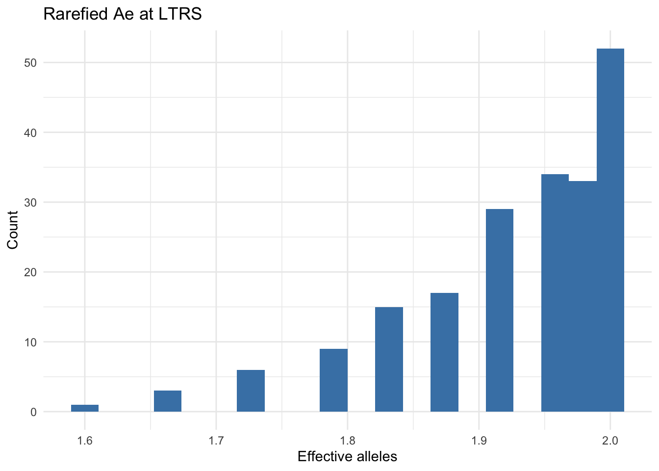

This is useful for comparing diversity across populations with unequal sample sizes.

4.6 Optimal Sampling

The optimal_sampling() function estimates how many individuals are needed to capture a given proportion of allelic diversity:

arapat |>
  pull(LTRS) |>
  optimal_sampling(nrep = 99)

4.7 Without Pipes

frequencies(arapat$LTRS)
frequencies(arapat, stratum = "Species")
frequencies(arapat, loci = c("LTRS", "WNT"))
frequency_matrix(arapat, stratum = "Species")
genotype_counts(arapat, stratum = "Species")
genotype_frequencies(arapat$LTRS)
hwe(arapat[arapat$Species == "Mainland", ])
rare_vals <- rarefaction(arapat$LTRS, mode = "Ae", size = 20, nperm = 199)
hist(rare_vals)
optimal_sampling(arapat$LTRS, nrep = 99)