5 Genetic Diversity

This chapter covers estimation of genetic diversity statistics using genetic_diversity(). As with genetic_structure(), genetic_distance() and genetic_relatedness(), this front-end function is the only way to reach the individual estimators; there are no standalone A(), He() or Fis() functions.

library(gstudio)
library(dplyr)
library(ggplot2)
data(arapat)

5.1 The `genetic_diversity()` Wrapper

The genetic_diversity() function is the main entry point for diversity estimation. It dispatches to specific estimators based on the mode parameter:

Mode	Statistic	Description
`"A"`	Allelic richness	Number of alleles
`"Ae"`	Effective alleles	\(1 / \sum p_i^2\)
`"A95"`	A (5% threshold)	Alleles with frequency >= 0.05
`"He"`	Expected heterozygosity	\(1 - \sum p_i^2\)
`"Ho"`	Observed heterozygosity	Proportion of heterozygotes
`"Hi"`	Individual heterozygosity	Proportion of an individual’s loci that are heterozygous
`"Hes"`	Corrected He	Nei’s unbiased within-stratum \(H_S\) (needs `stratum`)
`"Hos"`	Corrected Ho	Ho averaged across strata after Nei (needs `stratum`)
`"Ht"`	Total He	Nei’s unbiased total \(H_T\) (needs `stratum`)
`"Fis"`	Inbreeding coefficient	\(1 - H_o/H_e\)
`"Pe"`	Polymorphic index	\(\sum p_i(1-p_i)\)

5.2 Global (Unstratified) Estimates

Without a stratum, diversity is estimated across all individuals:

arapat |>
  genetic_diversity(mode = "A")

  Locus  A
1  LTRS  2
2   WNT  5
3    EN  5
4    EF  2
5   ZMP  2
6   AML 13
7  ATPS 10
8  MP20 19

arapat |>
  genetic_diversity(mode = "He")

  Locus        He
1  LTRS 0.4989034
2   WNT 0.6528320
3    EN 0.4489313
4    EF 0.4361538
5   ZMP 0.3394444
6   AML 0.8293685
7  ATPS 0.7193649
8  MP20 0.8185723

Pass several modes to get one table with a column for each:

arapat |>
  genetic_diversity(mode = c("A", "Ae", "He", "Ho"))

  Locus  A       Ae        He         Ho
1  LTRS  2 1.995623 0.4989034 0.23691460
2   WNT  5 2.880450 0.6528320 0.27840909
3    EN  5 1.814656 0.4489313 0.20555556
4    EF  2 1.773533 0.4361538 0.14404432
5   ZMP  2 1.513877 0.3394444 0.15454545
6   AML 13 5.860583 0.8293685 0.37058824
7  ATPS 10 3.563347 0.7193649 0.08539945
8  MP20 19 5.511837 0.8185723 0.44692737

5.3 Per-Stratum Estimates

Provide a stratum argument to compute diversity within each population:

arapat |>
  genetic_diversity(stratum = "Species", mode = "He")

     Stratum Locus         He
2       Cape  LTRS 0.14720000
3       Cape   WNT 0.23374726
4       Cape    EN 0.42000000
5       Cape    EF 0.06444444
6       Cape   ZMP 0.00000000
7       Cape   AML 0.53312835
8       Cape  ATPS 0.11546667
9       Cape  MP20 0.36791111
10  Mainland  LTRS 0.38850309
11  Mainland   WNT 0.03277778
12  Mainland    EN 0.50285714
13  Mainland    EF 0.27119377
14  Mainland   ZMP 0.09500000
15  Mainland   AML 0.53854875
16  Mainland  ATPS 0.25038580
17  Mainland  MP20 0.80670340
18 Peninsula  LTRS 0.42591805
19 Peninsula   WNT 0.50613781
20 Peninsula    EN 0.17229600
21 Peninsula    EF 0.48979592
22 Peninsula   ZMP 0.41492187
23 Peninsula   AML 0.72842417
24 Peninsula  ATPS 0.52255763
25 Peninsula  MP20 0.69148800

arapat |>
  genetic_diversity(stratum = "Species", mode = c("Ae", "He", "Fis"))

     Stratum Locus       Ae         He         Fis
1       Cape  LTRS 1.172608 0.14720000  0.27536232
2       Cape   WNT 1.305052 0.23374726  0.76875000
3       Cape    EN 1.724138 0.42000000  0.07936508
4       Cape    EF 1.068884 0.06444444  0.37931034
5       Cape   ZMP 1.000000 0.00000000         NaN
6       Cape   AML 2.141916 0.53312835  0.81506977
7       Cape  ATPS 1.130540 0.11546667  0.65357968
8       Cape  MP20 1.582056 0.36791111  0.52887171
9   Mainland  LTRS 1.635331 0.38850309 -0.21549156
10  Mainland   WNT 1.033889 0.03277778 -0.01694915
11  Mainland    EN 2.011494 0.50285714  0.54545455
12  Mainland    EF 1.372107 0.27119377 -0.19298246
13  Mainland   ZMP 1.104972 0.09500000  1.00000000
14  Mainland   AML 2.167076 0.53854875  0.73473684
15  Mainland  ATPS 1.334020 0.25038580  0.33436055
16  Mainland  MP20 5.173397 0.80670340  0.17359135
17 Peninsula  LTRS 1.741912 0.42591805  0.43166651
18 Peninsula   WNT 2.024856 0.50613781  0.25909507
19 Peninsula    EN 1.208161 0.17229600  0.14101314
20 Peninsula    EF 1.960000 0.48979592  0.69212963
21 Peninsula   ZMP 1.709173 0.41492187  0.48785539
22 Peninsula   AML 3.682213 0.72842417  0.35787148
23 Peninsula  ATPS 2.094494 0.52255763  0.83293405
24 Peninsula  MP20 3.241365 0.69148800  0.27692165

5.4 Single Loci

A bare locus vector can be passed in place of a data frame:

arapat |>
  pull(LTRS) |>
  genetic_diversity(mode = "Fis")

  Locus       Fis
1 Locus 0.5251293

5.5 Individual Heterozygosity

The Hi mode is estimated per individual rather than per locus. It returns one row for each individual, keeping the non-locus columns, so it can be summarized by any grouping you like:

arapat |>
  genetic_diversity(mode = "Hi") |>
  group_by(Species) |>
  summarize(mean_Hi = mean(Hi))

# A tibble: 3 × 2
  Species   mean_Hi
  <fct>       <dbl>
1 Cape        0.117
2 Mainland    0.301
3 Peninsula   0.275

5.6 Corrected Heterozygosity (Nei’s)

The Hes and Hos modes require a stratum because they apply a small-sample correction per subpopulation:

arapat |>
  genetic_diversity(stratum = "Species", mode = "Hes")

       Locus       Hes
1       LTRS 0.3233431
2        WNT 0.2606681
3         EN 0.3687470
4         EF 0.2781409
5        ZMP 0.1731159
6        AML 0.6108282
7       ATPS 0.2999070
8       MP20 0.6284672
9 Multilocus 0.3679022

Ht gives the matching total expected heterozygosity (the \(H_S\) and \(H_T\) that genetic_structure() builds \(G_{ST}\) from). These pooled modes return one row per locus, so they combine with each other but not with per-stratum modes:

arapat |>
  genetic_diversity(stratum = "Species", mode = c("Hos", "Hes", "Ht"))

       Locus        Hos       Hes        Ht
1       LTRS 0.27365079 0.3233431 0.4531627
2        WNT 0.15412913 0.2606681 0.6350801
3         EN 0.25441270 0.3687470 0.6561538
4         EF 0.17144102 0.2781409 0.3303420
5        ZMP 0.07083333 0.1731159 0.2039553
6        AML 0.23639688 0.6108282 0.8619706
7       ATPS 0.09798942 0.2999070 0.7548774
8       MP20 0.44666667 0.6284672 0.8734015
9 Multilocus 0.21318999 0.3679022        NA

5.7 Multilocus Diversity

The multilocus_diversity() function computes a summary across all loci:

arapat |>
  multilocus_diversity()

[1] 0.8374656

5.8 Selecting Specific Loci

You can restrict the analysis to a subset of loci, with or without a stratum:

arapat |>
  genetic_diversity(loci = c("LTRS", "WNT"), mode = "He")

  Locus        He
1  LTRS 0.4989034
2   WNT 0.6528320

or select the columns first:

arapat |>
  select(Species, LTRS, WNT) |>
  genetic_diversity(stratum = "Species", mode = "He")

    Stratum Locus         He
2      Cape  LTRS 0.14720000
3      Cape   WNT 0.23374726
4  Mainland  LTRS 0.38850309
5  Mainland   WNT 0.03277778
6 Peninsula  LTRS 0.42591805
7 Peninsula   WNT 0.50613781

5.9 Comparing Populations

A common workflow is to estimate diversity per population, then compare:

he_by_pop <- arapat |>
  genetic_diversity(stratum = "Species", mode = "He")

he_by_pop |>
  group_by(Stratum) |>
  summarize(mean_He = mean(He), sd_He = sd(He))

# A tibble: 3 × 3
  Stratum   mean_He sd_He
  <chr>       <dbl> <dbl>
1 Cape        0.235 0.188
2 Mainland    0.361 0.254
3 Peninsula   0.494 0.173

he_by_pop |>
  ggplot(aes(x = Stratum, y = He, fill = Stratum)) +
  geom_boxplot() +
  theme_minimal() +
  labs(title = "Expected Heterozygosity by Species",
       y = "He") +
  theme(legend.position = "none")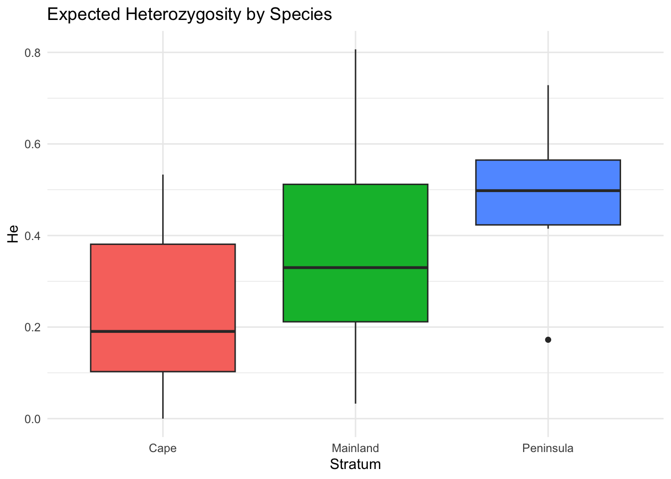

5.10 Without Pipes

genetic_diversity(arapat, mode = "He")
genetic_diversity(arapat, mode = c("A", "Ae", "He", "Ho"))
genetic_diversity(arapat, stratum = "Species", mode = "He")
genetic_diversity(arapat, loci = c("LTRS", "WNT"), mode = "He")
genetic_diversity(arapat$LTRS, mode = "Fis")
genetic_diversity(arapat, mode = "Hi")
multilocus_diversity(arapat)
he_by_pop <- genetic_diversity(arapat, stratum = "Species", mode = "He")
ggplot(he_by_pop, aes(x = Stratum, y = He, fill = Stratum)) +
  geom_boxplot()

5.1 The genetic_diversity() Wrapper