Study Area and Orthoimagery

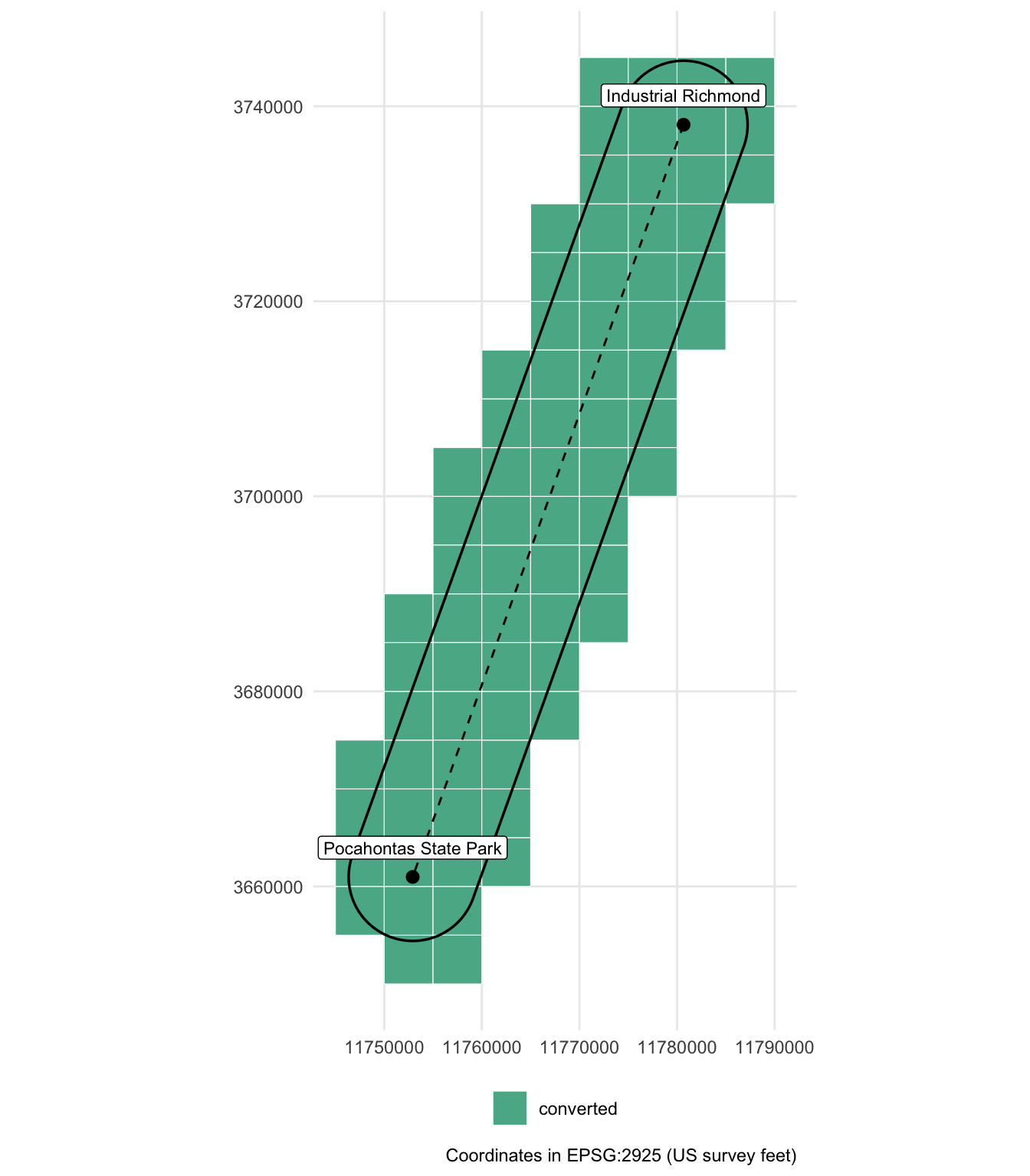
Transect from industrial Richmond to Pocahontas State Park

library(sf)
library(dplyr)
library(ggplot2)
library(leaflet)
library(yaml)
library(here)

cfg <- read_yaml(here("config.yml"))
derived <- here(cfg$paths$derived)

pts   <- st_read(file.path(derived, "aoi.gpkg"), layer = "transect_points", quiet = TRUE)
line  <- st_read(file.path(derived, "aoi.gpkg"), layer = "transect_line",   quiet = TRUE)
aoi   <- st_read(file.path(derived, "aoi.gpkg"), layer = "aoi",             quiet = TRUE)
tiles <- st_read(file.path(derived, "tiles_needed.gpkg"), quiet = TRUE)

# Status is checked at render time; tile paths are relative to the project root
tiles$converted <- file.exists(here(tiles$tif_path))
tiles$state <- case_when(
  tiles$converted          ~ "converted",
  tiles$status == "local"  ~ "local (not converted)",
  TRUE                     ~ "missing (download needed)"
)
state_cols <- c("converted" = "#1b9e77",
                "local (not converted)" = "#7570b3",
                "missing (download needed)" = "#d95f02")

Purpose

This project uses 2025 Virginia Base Mapping Program (VBMP) orthoimagery along a transect from industrial Richmond to Pocahontas State Park. The statewide imagery is distributed as RGB MrSID tiles, and VGIN supplies 4-band (red, green, blue, near-infrared) GeoTIFF tiles on request. Only the tiles that overlap the study area are used, combined into a single virtual mosaic. The mosaic is built from the 4-band GeoTIFFs (imagery_source: "4band" in config.yml), so it carries the near-infrared band needed for NDVI.

Step	Script	Output
1. Build transect and buffer	R/01_build_aoi.R	data/derived/aoi.gpkg
2. Select intersecting tiles	R/02_select_tiles.R	data/derived/tiles_needed.{gpkg,csv}
3. Convert MrSID to GeoTIFF (RGB only; not needed with the 4-band tiles)	python/convert_mrsid.py (QGIS Python console)	data/geotiff/*.tif
4. Virtual mosaic	R/03_build_vrt.R	data/derived/ortho_12in.vrt, ortho_12in_preview.tif

All parameters live in config.yml. Analysis scripts load the imagery with load_ortho() from R/functions.R, which returns the mosaic limited to the study area without copying any data.

Study area

len_km  <- as.numeric(line$length_km)
area_km <- as.numeric(aoi$area_km2)

• Start: Industrial Richmond (37.584817° N, 77.472433° W)
• End: Pocahontas State Park (37.373768° N, 77.570813° W)
• Transect length: 24.99 km
• Buffer: 2 km each side, round end caps
• Study area: 112.5 km²
• CRS: EPSG:2925 (NAD83(HARN) / Virginia South (ftUS))

to_ll <- function(x) st_transform(x, 4326)
pal <- colorFactor(unname(state_cols), levels = names(state_cols))

leaflet() |>
  addProviderTiles(providers$Esri.WorldImagery, group = "Imagery") |>
  addProviderTiles(providers$Esri.WorldGrayCanvas, group = "Light") |>
  addPolygons(data = to_ll(tiles), color = "white", weight = 1,
              fillColor = ~pal(state), fillOpacity = 0.4,
              label = ~paste0(tile_name, " (", state, ")"), group = "Tiles") |>
  addPolygons(data = to_ll(aoi), color = "black", weight = 2, fill = FALSE, group = "Study area") |>
  addPolylines(data = to_ll(line), color = "black", dashArray = "6", weight = 2) |>
  addCircleMarkers(data = to_ll(pts), radius = 5, color = "black", label = ~name) |>
  addLegend(pal = pal, values = names(state_cols), title = "Tile status") |>
  addLayersControl(baseGroups = c("Imagery", "Light"), overlayGroups = c("Tiles", "Study area"))

Orthoimagery tiles

Tiles were selected by intersecting the study area with the VBMP 2025 12-inch tile index footprints (South and North state plane zones searched).

tiles |>
  st_drop_geometry() |>
  count(state, name = "tiles") |>
  knitr::kable(col.names = c("Status", "Tiles"))

Status	Tiles
converted	75

ggplot() +
  geom_sf(data = tiles, aes(fill = state), colour = "white", linewidth = 0.2, alpha = 0.8) +
  geom_sf(data = aoi, fill = NA, colour = "black", linewidth = 0.6) +
  geom_sf(data = line, colour = "black", linetype = "dashed") +
  geom_sf(data = pts, size = 2.5) +
  geom_sf_label(data = pts, aes(label = name), nudge_y = 3000, size = 3) +
  scale_fill_manual(values = state_cols, name = NULL) +
  coord_sf(datum = st_crs(cfg$crs)) +
  labs(x = NULL, y = NULL, caption = "Coordinates in EPSG:2925 (US survey feet)") +
  theme_minimal() +
  theme(legend.position = "bottom")

Tiles required to reproduce

To rebuild the data, download these MrSID tiles (.sid and .sdw) from the VGIN VBMP site into data/raw/tiles/.

tiles |>
  st_drop_geometry() |>
  mutate(section = sub("^DO_(S\\d+_\\d{4})_.*", "\\1", tile_name),
         quarter = sub("^DO_S\\d+_\\d{4}_(\\d+)\\..*", "\\1", tile_name)) |>
  group_by(section) |>
  summarise(tiles = n(), quarters = paste(quarter, collapse = ", ")) |>
  knitr::kable(col.names = c("Section", "Tiles", "Quarter codes"))

Section	Tiles	Quarter codes
S13_7645	1	30
S13_7646	2	30, 40
S13_7647	1	40
S13_7655	4	10, 20, 30, 40
S13_7656	4	10, 20, 30, 40
S13_7657	4	10, 20, 30, 40
S13_7658	4	10, 20, 30, 40
S13_7659	2	30, 40
S13_7666	2	10, 20
S13_7667	3	10, 20, 30
S13_7668	4	10, 20, 30, 40
S13_7669	4	10, 20, 30, 40
S13_7678	1	20
S13_7679	2	10, 20
S13_7750	1	40
S13_7760	4	10, 20, 30, 40
S13_7761	3	10, 30, 40
S13_7762	2	30, 40
S13_7770	4	10, 20, 30, 40
S13_7771	4	10, 20, 30, 40
S13_7772	4	10, 20, 30, 40
S13_7773	4	10, 20, 30, 40
S13_7774	2	10, 40
S13_7781	1	20
S13_7782	2	10, 20
S13_7783	4	10, 20, 30, 40
S13_7784	2	10, 40

log_path <- file.path(derived, "conversion_log.csv")
if (file.exists(log_path)) {
  log <- read.csv(log_path)
  cat(sprintf("**Conversion:** %d of %d tiles converted to GeoTIFF (%d errors logged).",
              sum(tiles$converted), nrow(tiles), sum(log$result == "error")))
} else {
  cat(sprintf("**Conversion:** %d of %d tiles converted to GeoTIFF.",
              sum(tiles$converted), nrow(tiles)))
}

Conversion: 75 of 75 tiles converted to GeoTIFF (0 errors logged).

Mosaic

vrt_path     <- file.path(derived, "ortho_12in.vrt")
preview_path <- file.path(derived, "ortho_12in_preview.tif")
has_mosaic   <- file.exists(vrt_path) && file.exists(preview_path)

ortho <- terra::rast(vrt_path)
preview <- terra::rast(preview_path)
cat(sprintf(
  "The virtual mosaic combines %d GeoTIFF tiles into one %s × %s px image at %g ft resolution
  (bands: %s). It only references the tiles, so it takes no extra disk space.
  The preview below is resampled to %g ft pixels; the study area is outlined in yellow.",
  nrow(tiles), format(terra::ncol(ortho), big.mark = ","), format(terra::nrow(ortho), big.mark = ","),
  terra::res(ortho)[1], paste(names(ortho), collapse = ", "), terra::res(preview)[1]
))

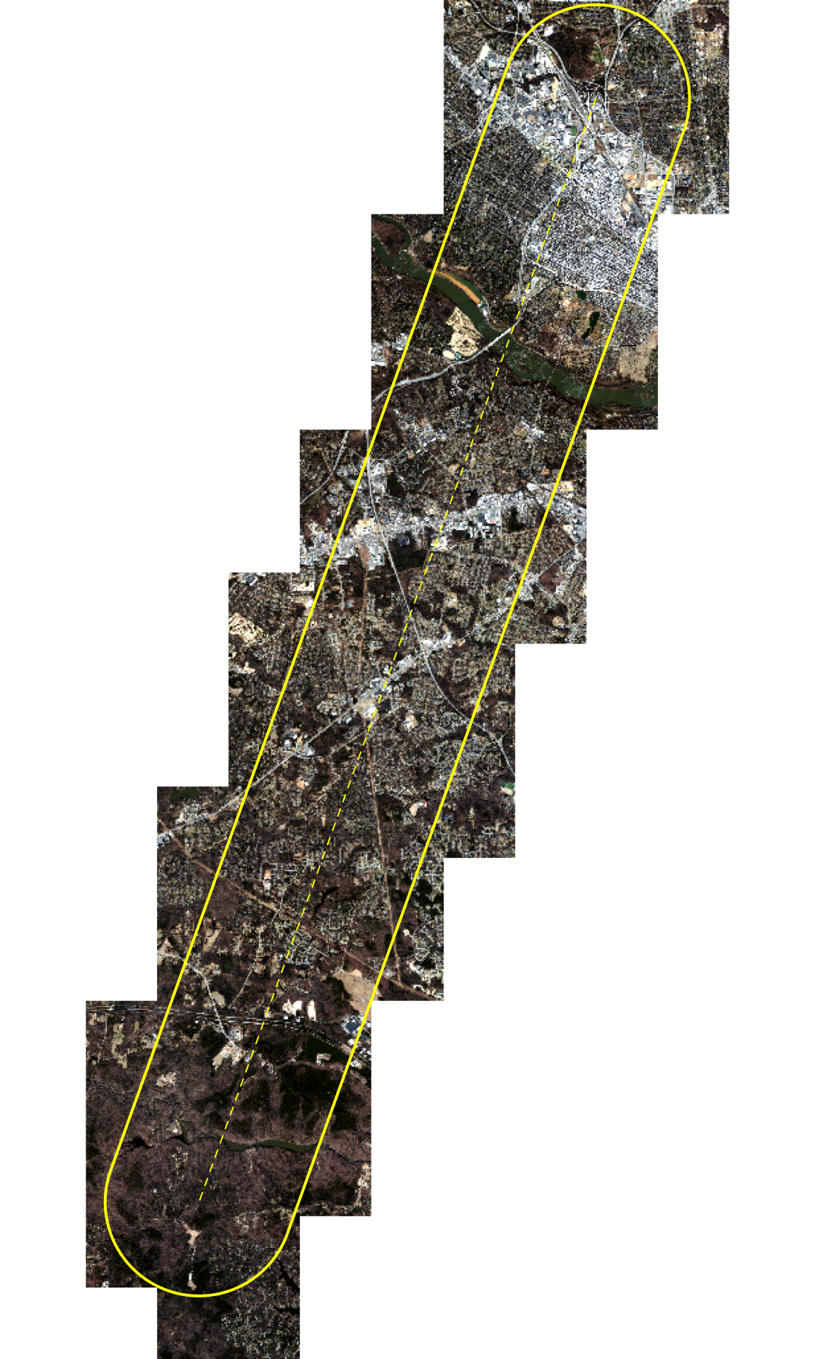
The virtual mosaic combines 75 GeoTIFF tiles into one 45,000 × 95,000 px image at 1 ft resolution (bands: red, green, blue, nir). It only references the tiles, so it takes no extra disk space. The preview below is resampled to 25 ft pixels; the study area is outlined in yellow.

terra::plotRGB(preview, stretch = "lin", mar = c(0, 0, 0, 0))
terra::plot(terra::vect(aoi), add = TRUE, border = "yellow", lwd = 2)
terra::plot(terra::vect(line), add = TRUE, col = "yellow", lty = 2)

Notes

• Imagery source: VBMP 2025 12-inch orthoimagery (Sanborn Map Company, flown February to March 2025), distributed by the Virginia Geographic Information Network (VGIN). The MrSID versions are RGB only. The near-infrared band is only in the 4-band GeoTIFF deliverables, which share the MrSID tiles’ names and pixel grid exactly (same 5,000 × 5,000 px extent and origin, EPSG:2925). Their RGB bands are the uncompressed originals: compared with the MrSID-derived RGB they differ by about 5 digital numbers on average, with no bias (MrSID compression noise), so the 4-band tiles replace the MrSID set.
• Tile layout: each 12-inch tile is 5,000 × 5,000 px at 1 ft, covering 5,000 × 5,000 ft. Tile names follow DO_S13_<section>_<quarter>.2025.
• MrSID decoding (only needed with imagery_source: "rgb"): the MrSID GDAL driver only loads inside the QGIS application (macOS code-signing blocks it from the command line), so conversion runs in the QGIS Python console.
• Mosaic edges: the VRT has no nodata value. Areas outside the tiles read as 0 in all bands; all such areas lie outside the study area.