Holly Candidates

Small, isolated evergreen crowns in leaf-off imagery as candidate holly locations

Published

November 4, 2026

Code

library(sf)
library(dplyr)
library(tidyr)
library(ggplot2)
library(leaflet)
library(plotly)
library(terra)
library(here)

source(here("R", "functions.R"))
derived <- here(cfg$paths$derived)
h <- cfg$holly

line    <- load_transect()
windows <- load_windows()
obj     <- holly_candidates(load_holly_objects())
# Earlier runs kept for comparison: RGB only (GLI) and plain NDVI (shadow-biased)
read_run <- function(f) {
  f <- file.path(derived, f)
  if (file.exists(f)) holly_candidates(st_read(f, quiet = TRUE)) else NULL
}
obj_gli  <- read_run("holly_objects_gli.gpkg")
obj_ndvi <- read_run("holly_objects_ndvi.gpkg")
curve_path <- file.path(derived, "ndvi_shadow_curve.csv")
curve   <- if (file.exists(curve_path)) read.csv(curve_path) else NULL
cal_path <- file.path(derived, "ndvi_calibration.csv")
cal     <- if (file.exists(cal_path)) read.csv(cal_path) else NULL
classes <- read.csv(file.path(derived, "nlcd_window_classes.csv"))
nlcd    <- read.csv(file.path(derived, "nlcd_windows.csv"))

vi_name <- unique(obj$vi_name)
index_labels <- c(gli = "GLI (green leaf index, RGB)", ndvi = "NDVI (near-infrared)",
                  ndvi_adj = "brightness-adjusted NDVI")
vi_label <- index_labels[vi_name]
thr <- h$thresholds[[vi_name]]

reason_cols <- c(candidate = "#d95f02", `not isolated` = "#7570b3",
                 `developed/water` = "#999999", size = "#cccccc")

Candidates now use brightness-adjusted NDVI

The candidates on this page come from NDVI computed from the 4-band (RGB + near-infrared) imagery, adjusted for brightness because plain NDVI is inflated in shadow (see Shadows). Two earlier runs are kept for comparison in GLI versus NDVI: the RGB-only green leaf index (GLI) and plain NDVI. Candidates are still unverified: until field data exist, they are locations to visit, not holly.

Purpose

American holly (Ilex opaca) is evergreen, so in leaf-off imagery (flown February to March 2025) its crowns stay green while the deciduous canopy around it is bare. This page builds the first step of a holly classification workflow:

Candidates from imagery (this page): find small, isolated evergreen crowns in non-developed areas.
Ground truth: visit candidate locations and record what is there (holly, sex if known, or the false-positive species).
Classification: train a supervised classifier on crown features (including NDVI and NIR) using the field labels, then map holly across the transect.

Step	Script	Output
7. Crown extraction	`R/06_holly_objects.R`	`data/derived/holly_objects.gpkg` (all crowns with features)
8. Candidate rule	`holly_candidates()` in `R/functions.R`	`data/derived/holly_candidates.{csv,gpx}` (field list)

Greenness comes from brightness-adjusted NDVI. The mosaic is built from the 4-band tiles, and veg_index() uses it whenever the imagery has a nir band (GLI otherwise). Every crown also records its mean GLI and plain NDVI, so the indices can be compared on the same objects.

Why NDVI

Healthy leaves treat red and near-infrared (NIR) light very differently. Chlorophyll absorbs most red light for photosynthesis, while the internal cell structure of a leaf (the spongy mesophyll) scatters and reflects most NIR light. Bare branches, dead or dormant grass, soil, and pavement show much less of this contrast. The normalized difference vegetation index captures it in one number:

\[ \text{NDVI} = \frac{\text{NIR} - \text{Red}}{\text{NIR} + \text{Red}} \]

NDVI ranges from −1 to 1. Water is negative, soil, rock, and pavement sit near 0, and dense green foliage is typically above 0.6. Because it is a ratio, it is also less sensitive to illumination than a single band, so a shaded crown and a sunlit crown of the same tree give similar values.

This contrast is what makes leaf-off imagery useful for holly. In February and March the deciduous canopy is bare and has low NDVI, while evergreen foliage stays green and has high NDVI. Holly in the understory should stand out clearly against the bare hardwoods around it.

The RGB stand-in used for the first pass, the green leaf index (GLI), relies only on the small green reflectance peak of leaves in visible light. In this imagery GLI separates pine canopy (median about 0.03) from leaf-off hardwood (about −0.01) by only a narrow margin. It is also affected by shadows and by the imagery’s slight blue cast.

Separation in this imagery

To compare the indices and set thresholds, each was computed (3 × 3 px smoothed, as in crown extraction) at 60,000 random points in the study area and grouped by NLCD class (R/05b_ndvi_calibration.R). NLCD is a 30 m product, so these labels are noisy at 1 ft (a “deciduous” cell can contain a pine or a holly), which blurs every index.

Code

auc <- function(neg, pos) {
  r <- rank(c(neg, pos))
  (sum(r[length(neg) + seq_along(pos)]) - length(pos) * (length(pos) + 1) / 2) /
    (length(neg) * length(pos))
}
dec <- cal[cal$nlcd %in% 41, ]
evg <- cal[cal$nlcd %in% 42, ]
ix <- intersect(c("gli", "ndvi", "ndvi_adj"), names(cal))
cal_tab <- do.call(rbind, lapply(ix, function(k) data.frame(
  Index = index_labels[[k]],
  dec = median(dec[[k]], na.rm = TRUE), evg = median(evg[[k]], na.rm = TRUE),
  crown = h$thresholds[[k]]$crown,
  dec_over = mean(dec[[k]] > h$thresholds[[k]]$crown, na.rm = TRUE),
  dark_over = mean(dec[[k]][dec$brightness < 60] > h$thresholds[[k]]$crown, na.rm = TRUE),
  evg_over = mean(evg[[k]] > h$thresholds[[k]]$crown, na.rm = TRUE),
  auc = auc(dec[[k]], evg[[k]]))))
knitr::kable(cal_tab, digits = c(0, 2, 2, 2, 3, 3, 3, 2), row.names = FALSE,
             col.names = c("Index", "Median, deciduous (41)", "Median, evergreen (42)",
                           "Crown threshold", "Deciduous above", "Shaded deciduous above",
                           "Evergreen above", "AUC"))

Index	Median, deciduous (41)	Median, evergreen (42)	Crown threshold	Deciduous above	Shaded deciduous above	Evergreen above	AUC
GLI (green leaf index, RGB)	-0.01	0.03	0.05	0.025	0.016	0.343	0.77
NDVI (near-infrared)	0.33	0.58	0.60	0.021	0.293	0.423	0.90
brightness-adjusted NDVI	-0.12	1.38	1.70	0.053	0.039	0.297	0.84

AUC is the probability that a random evergreen-forest point has a higher index than a random deciduous-forest point (0.5 = no separation, 1 = complete). “Shaded deciduous above” is the false-positive rate among deciduous-forest points darker than 60 (mean of the RGB bands, 0–255). NDVI separates the forest types much better than GLI, but most of its apparent advantage in the shade is an artifact, as the next section shows.

Shadows

Code

bins <- cal |>
  filter(nlcd %in% c(41, 42), brightness >= 30, brightness < 160) |>
  mutate(cover = factor(nlcd, c(41, 42), c("Deciduous forest (41)", "Evergreen forest (42)")),
         b = 10 * floor(brightness / 10) + 5) |>
  group_by(cover, b) |>
  filter(n() >= 20) |>
  summarise(ndvi = median(ndvi), ndvi_adj = median(ndvi_adj), .groups = "drop") |>
  pivot_longer(c(ndvi, ndvi_adj), names_to = "index") |>
  mutate(index = c(ndvi = "Plain NDVI", ndvi_adj = "Brightness-adjusted NDVI (SD units)")[index])
thr_lines <- data.frame(index = c("Plain NDVI", "Brightness-adjusted NDVI (SD units)"),
                        v = c(h$thresholds$ndvi$crown, h$thresholds$ndvi_adj$crown))
ggplot(bins, aes(b, value, colour = cover)) +
  geom_line(linewidth = 0.8) + geom_point(size = 1.5) +
  geom_hline(data = thr_lines, aes(yintercept = v), linetype = "dashed") +
  facet_wrap(~index, scales = "free_y") +
  scale_colour_manual(values = c("#b5651d", "#1b7837"), name = NULL) +
  labs(x = "Brightness (mean of RGB, 0–255; shadow at left)", y = "Median (dashed: crown threshold)") +
  theme_minimal() +
  theme(legend.position = "top", panel.grid.minor = element_blank())

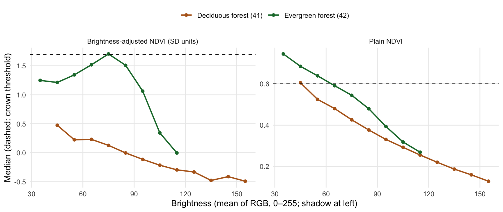
Plain NDVI rises steadily as pixels get darker. In leaf-off deciduous forest the median is about 0.2 for bright pixels and about 0.6 in shadow, the same as evergreen foliage: in shadow the red band falls nearly to zero while the NIR band stays high, lit by light scattered from the surrounding vegetation. A fixed NDVI threshold therefore picks up tree and building shadows. The first NDVI run did exactly this: its candidates were much darker than GLI’s, and many were shadows.

The brightness-adjusted NDVI compares each pixel with leaf-off deciduous forest at the same brightness:

\[ \text{NDVI}_\text{adj} = \frac{\text{NDVI} - \mu(b)}{\sigma(b)} \]

where b is brightness and μ(b) and σ(b) are the mean and spread of NDVI in NLCD deciduous forest at that brightness (loess fits, saved in data/derived/ndvi_shadow_curve.csv). It is in units of deciduous-forest standard deviations: about 0 for bare hardwood at any brightness, positive for foliage greener than leaf-off forest. Dividing by σ(b) matters because NDVI is also noisier in shadow; subtracting the mean alone still let about 20% of shaded deciduous pixels through.

The crown threshold (1.7) is exceeded by about 5% of deciduous-forest pixels at every brightness, and the context threshold (1) by about 15%. The price is that evergreen foliage in deep shadow can no longer be told from shaded hardwood. That is a real limit of this imagery, not of the method: a shaded holly is invisible to both indices. Overall AUC drops a little because part of plain NDVI’s apparent separation came from evergreen canopy being darker than deciduous canopy, which is the shadow effect again.

Measuring the gain from NIR

Every crown carries GLI, plain NDVI, and the adjusted index (gli_mean, ndvi_mean, vi_mean) along with mean band values, including NIR. Once field labels exist, the comparison will use the same ground-truth set and the same spatially blocked cross-validation for two classifiers:

Visible only: crown features from RGB (GLI, colour, brightness, size, shape, isolation).
Visible + NIR: the same features plus NDVI and NIR reflectance.

The improvement will be reported as the change in precision (share of candidates that are holly), recall (share of holly found), and overall accuracy, along with how many candidates drop out of the field list.

Approach

Each 12-inch tile is processed at full resolution:

Vegetation index (brightness-adjusted NDVI), smoothed with a 3 × 3 px mean.
Crowns: pixels with index > 1.7 are evergreen crown; connected groups of them are crown objects. Objects 6–30 ft across (equivalent-circle diameter) are kept with their features.
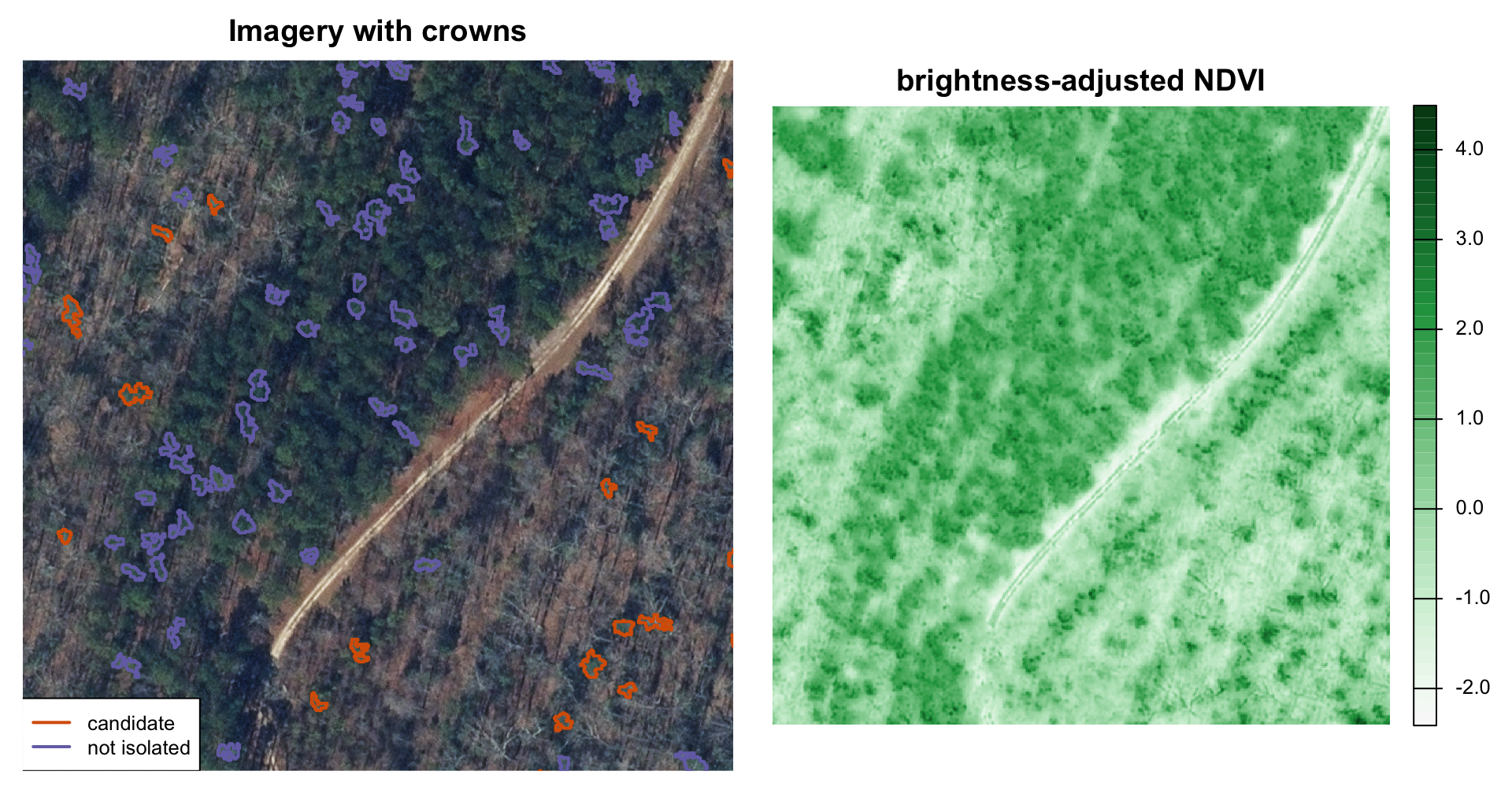
Isolation: the share of evergreen pixels (index > 1, a lower threshold) in the 70 ft neighbourhood of each crown. Holly in a leaf-off hardwood stand has a low share; a crown inside pine canopy has a high one.
Candidate rule: crown 10–20 ft across, evergreen share ≤ 0.25, and NLCD class not water or developed (11, 21, 22, 23, 24). Crowns cut by a tile edge are excluded from the field list.

Thresholds are calibrated on NLCD forest classes (see Separation in this imagery and Shadows).

Example

A 600 × 600 ft area 22.5 km along the transect: a pine stand (upper left) next to leaf-off hardwoods (lower right). Candidates are the isolated crowns in the hardwood stand; crowns inside the pine canopy are rejected as not isolated.

Code

ends <- st_coordinates(line)[, 1:2]
d <- (ends[2, ] - ends[1, ]) / sqrt(sum((ends[2, ] - ends[1, ])^2))
p <- ends[1, ] + km_to_crs(22.5) * d
e <- ext(p[1] - 300, p[1] + 300, p[2] - 300, p[2] + 300)
chip <- crop(load_ortho(aoi = FALSE), e)
names(chip) <- band_names(chip)
vi <- focal(veg_index(chip, vi_name), h$smooth_px, "mean", na.policy = "omit")
ex <- obj[st_as_sf(as.polygons(e, crs = crs(chip))), ]
ex <- ex[ex$reason %in% c("candidate", "not isolated"), ]

par(mfrow = c(1, 2), mar = c(0.5, 0.5, 2, 0.5))
plotRGB(chip, mar = c(0.5, 0.5, 2, 0.5)); title("Imagery with crowns")
plot(vect(ex), add = TRUE, border = reason_cols[ex$reason], lwd = 2)
legend("bottomleft", c("candidate", "not isolated"), col = reason_cols[c("candidate", "not isolated")],
       lwd = 2, bg = "white", cex = 0.8)
plot(vi, main = vi_label, axes = FALSE, legend = TRUE, mar = c(0.5, 0.5, 2, 4),
     col = hcl.colors(50, "Greens 3", rev = TRUE))

Candidates

Code

n_tot <- nrow(obj)
n_cand <- sum(obj$candidate & !obj$tile_edge)
obj |>
  st_drop_geometry() |>
  mutate(reason = factor(reason, levels = names(reason_cols))) |>
  count(reason, name = "crowns") |>
  mutate(share = sprintf("%.1f%%", 100 * crowns / sum(crowns))) |>
  knitr::kable(col.names = c("Rule outcome", "Crowns", "Share"),
               format.args = list(big.mark = ","))

Rule outcome	Crowns	Share
candidate	12,814	4.8%
not isolated	47,597	17.8%
developed/water	46,414	17.3%
size	161,200	60.1%

Of 268,025 evergreen crowns 6–30 ft across in the study area, 12,814 pass the candidate rule (the outcome is the first rule a crown fails). Zoom in on the map to see individual candidates over the imagery; click one for its id and features.

Code

cand <- obj[obj$candidate & !obj$tile_edge, ]
cand_ll <- st_transform(st_centroid(cand), 4326)
cand_ll$popup <- sprintf(
  "<b>%s</b><br>%.0f ft crown<br>%s %.3f<br>Evergreen share: %.2f<br>Window %d (%.1f km)<br>%.6f, %.6f",
  cand_ll$obj_id, cand_ll$diam_ft, toupper(vi_name), cand_ll$vi_mean, cand_ll$context,
  cand_ll$window, cand_ll$u_km, cand_ll$lat, cand_ll$lon
)

leaflet(cand_ll) |>
  addProviderTiles(providers$Esri.WorldImagery, group = "Imagery",
                   options = providerTileOptions(maxNativeZoom = 19, maxZoom = 21)) |>
  addProviderTiles(providers$Esri.WorldGrayCanvas, group = "Light") |>
  addPolylines(data = st_transform(line, 4326), color = "white", dashArray = "6", weight = 2) |>
  addCircleMarkers(radius = 5, color = "#d95f02", weight = 2, fillOpacity = 0.3,
                   popup = ~popup, clusterOptions = markerClusterOptions(disableClusteringAtZoom = 18)) |>
  addLayersControl(baseGroups = c("Imagery", "Light"))

Along the transect

Candidate density per km² of non-developed land (NLCD classes other than 11, 21, 22, 23, 24) in each 1 km window, with the window’s forest cover for reference.

Code

nondev <- classes |>
  filter(!class %in% h$exclude_nlcd) |>
  group_by(window) |>
  summarise(nondev_frac = sum(frac))
dens <- windows |>
  st_drop_geometry() |>
  left_join(nondev, by = "window") |>
  left_join(count(st_drop_geometry(cand), window, name = "n"), by = "window") |>
  left_join(select(nlcd, window, forest_pct), by = "window") |>
  mutate(n = coalesce(n, 0L),
         nondev_km2 = area_km2 * nondev_frac,
         per_km2 = ifelse(nondev_km2 > 0.05, n / nondev_km2, NA))

plot_ly(dens, x = ~u_mid_km) |>
  add_bars(y = ~per_km2, name = "Candidates per km² non-developed",
           marker = list(color = "#d95f02"),
           customdata = ~sprintf("%d candidates in %.2f km²", n, nondev_km2),
           hovertemplate = "%{y:.0f} per km² (%{customdata})<extra></extra>") |>
  layout(xaxis = list(title = "Distance from Richmond (km)", dtick = 5),
         yaxis = list(title = "Candidates per km²"),
         hovermode = "x unified", showlegend = FALSE) |>
  config(displaylogo = FALSE)

Candidate gallery

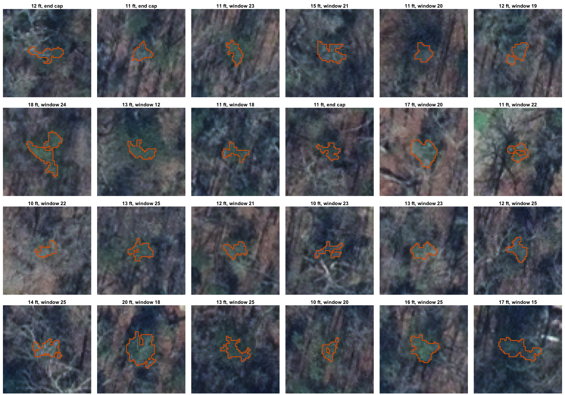
A random sample of candidates, 60 × 60 ft around each crown (outlined), for a quick visual check of what the rule picks up.

Code

set.seed(2025)
ortho <- load_ortho(aoi = FALSE)
samp <- cand[sample(nrow(cand), min(24, nrow(cand))), ]
par(mfrow = c(4, 6), mar = c(0.2, 0.2, 1.2, 0.2))
for (i in seq_len(nrow(samp))) {
  ctr <- st_coordinates(st_centroid(st_geometry(samp[i, ])))
  x <- crop(ortho, ext(ctr[1] - 30, ctr[1] + 30, ctr[2] - 30, ctr[2] + 30))
  plotRGB(x[[1:3]], mar = c(0.2, 0.2, 1.2, 0.2))
  plot(vect(samp[i, ]), add = TRUE, border = "#d95f02", lwd = 1.5)
  where <- if (is.na(samp$window[i])) "end cap" else sprintf("window %d", samp$window[i])
  title(sprintf("%.0f ft, %s", samp$diam_ft[i], where), cex.main = 0.8, line = 0.2)
}

Crown features

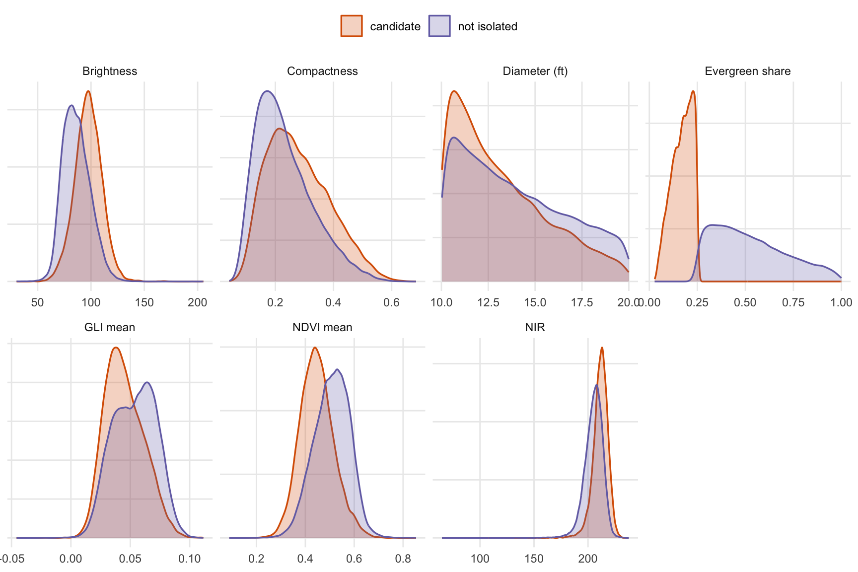
Features recorded for every crown, compared between candidates and crowns rejected as not isolated (mostly crowns within pine or other evergreen canopy). These are the starting inputs for the classifier.

Code

obj |>
  st_drop_geometry() |>
  filter(reason %in% c("candidate", "not isolated")) |>
  select(reason, any_of(c(`Diameter (ft)` = "diam_ft", Compactness = "compactness",
                          `NDVI mean` = "ndvi_mean", `GLI mean` = "gli_mean", NIR = "nir",
                          Brightness = "brightness", `Evergreen share` = "context"))) |>
  pivot_longer(-reason) |>
  ggplot(aes(value, fill = reason, colour = reason)) +
  geom_density(alpha = 0.25, linewidth = 0.6) +
  facet_wrap(~name, scales = "free", nrow = 2) +
  scale_fill_manual(values = reason_cols, name = NULL) +
  scale_colour_manual(values = reason_cols, name = NULL) +
  labs(x = NULL, y = NULL) +
  theme_minimal() +
  theme(legend.position = "top", axis.text.y = element_blank(), panel.grid.minor = element_blank())

GLI versus NDVI

Code

runs <- list(GLI = obj_gli, NDVI = obj_ndvi, `NDVI adjusted` = obj)
cands <- lapply(runs, function(o) o[o$candidate & !o$tile_edge, ])
match_ft <- 10    # candidates "match" if their centres are this close
near <- function(a, b) lengths(st_is_within_distance(st_centroid(st_geometry(a)),
                                                     st_centroid(st_geometry(b)), match_ft)) > 0
fmt <- function(x) format(x, big.mark = ",")
pct <- function(k) sprintf("%s (%.0f%%)", fmt(sum(k)), 100 * mean(k))
in_adj <- lapply(cands, near, b = cands[["NDVI adjusted"]])
cmp <- data.frame(
  Measure = c("Crowns extracted (6–30 ft)", "Candidates (field list)",
              sprintf("Also a candidate with adjusted NDVI (within %d ft)", match_ft),
              "Median candidate diameter (ft)", "Median candidate brightness (0–255)",
              "Median evergreen share around candidates"),
  check.names = FALSE,
  sapply(names(runs), function(k) c(
    fmt(nrow(runs[[k]])), fmt(nrow(cands[[k]])),
    if (k == "NDVI adjusted") "" else pct(in_adj[[k]]),
    sprintf("%.1f", median(cands[[k]]$diam_ft)),
    sprintf("%.0f", median(cands[[k]]$brightness)),
    sprintf("%.2f", median(cands[[k]]$context))))
)

The same crown extraction and candidate rule, run with each index. Thresholds for GLI and plain NDVI were matched on deciduous-forest false positives; the adjusted index holds that rate constant across brightness.

Code

knitr::kable(cmp, align = "lrrr")

Measure	GLI	NDVI	NDVI adjusted
Crowns extracted (6–30 ft)	177,671	155,299	268,025
Candidates (field list)	9,405	5,274	12,814
Also a candidate with adjusted NDVI (within 10 ft)	3,451 (37%)	1,000 (19%)
Median candidate diameter (ft)	13.3	12.5	12.6
Median candidate brightness (0–255)	82	54	97
Median evergreen share around candidates	0.18	0.18	0.18

Code

bind_rows(lapply(runs, function(o) st_drop_geometry(o)[, "reason", drop = FALSE]), .id = "index") |>
  mutate(reason = factor(reason, levels = names(reason_cols)),
         index = factor(index, names(runs))) |>
  count(index, reason) |>
  pivot_wider(names_from = index, values_from = n) |>
  knitr::kable(col.names = c("Rule outcome", paste(names(runs), "crowns")),
               format.args = list(big.mark = ","))

Rule outcome	GLI crowns	NDVI crowns	NDVI adjusted crowns
candidate	9,405	5,274	12,814
not isolated	21,658	26,079	47,597
developed/water	40,540	32,073	46,414
size	106,068	91,873	161,200

Code

run_cols <- c(GLI = "#999999", NDVI = "#7570b3", `NDVI adjusted` = "#d95f02")
cmp_dens <- bind_rows(lapply(cands, function(cc) count(st_drop_geometry(cc), window)), .id = "index") |>
  right_join(tidyr::expand_grid(index = names(runs), select(dens, window, u_mid_km, nondev_km2)),
             by = c("index", "window")) |>
  mutate(n = coalesce(n, 0L), per_km2 = ifelse(nondev_km2 > 0.05, n / nondev_km2, NA)) |>
  arrange(index, u_mid_km)

p <- plot_ly()
for (k in names(runs)) {
  p <- add_trace(p, data = filter(cmp_dens, index == k), x = ~u_mid_km, y = ~per_km2,
                 type = "scatter", mode = "lines+markers", name = k,
                 line = list(color = run_cols[[k]], width = 2),
                 marker = list(color = run_cols[[k]], size = 7),
                 hovertemplate = paste0(k, ": %{y:.0f} per km²<extra></extra>"))
}
p |>
  layout(xaxis = list(title = "Distance from Richmond (km)", dtick = 5, hoverformat = ".1f"),
         yaxis = list(title = "Candidates per km² non-developed", rangemode = "tozero"),
         hovermode = "x unified", legend = list(orientation = "h", y = -0.2)) |>
  config(displaylogo = FALSE)

What changed.

GLI (RGB only) found crowns that look green in RGB, including green-tinted bark, litter, and moss with no near-infrared signal of live foliage.
Plain NDVI swapped that error for a worse one: its candidates are the darkest of the three runs (see brightness above), and the gallery for that run was dominated by tree and building shadows.
Adjusted NDVI candidates are mid-brightness crowns that are greener than leaf-off forest in both RGB (median GLI 0.04) and NIR. It shares more candidates with GLI (37% of GLI candidates) than with plain NDVI (19%), which is consistent with plain NDVI’s extra candidates being shadows. The gallery above shows sunlit green crowns in leaf-off hardwood, the pattern expected for understory evergreens.

The adjusted index yields the most candidates of the three, because its crown threshold admits 5% of deciduous-forest pixels (versus about 2% for the other two) to keep enough evergreen foliage above it once shadows no longer help. The rule can be tightened at render time (candidate_diam_ft, context_max in config.yml) if the field list is too long, but field results should guide that rather than the count alone.

Across all three runs candidate density rises from Richmond toward Pocahontas State Park, so the gradient itself does not depend on the index. Which list actually finds holly is a question for the field visits.

Ground truth

The field list is data/derived/holly_candidates.csv (with a GPX copy for GPS units and phone apps). Each row has the crown id, latitude and longitude, transect position, crown diameter, and the features used by the rule. Suggested field record per visited candidate:

Field	Values
`obj_id`	crown id from the list (or new id for holly found nearby but not listed)
`species`	Ilex opaca, or the false positive (e.g. eastern red cedar, pine, magnolia, privet, ivy-covered trunk, lawn)
`sex`	female (fruit), male, unknown
`dbh_cm`, `height_m`	optional size measures
`notes`, `photo`	free text and photo id

Crown ids are tied to the current thresholds; if the rule or index changes, match field records to crowns by location rather than id. Keep field data outside data/derived/ (for example data/field/), since derived files are rebuilt by the scripts.

Next steps

Sampling design: a stratified random sample of candidates per window (or per NLCD class), so the field effort covers the full gradient. To learn which index works, the visit list should also include a small random sample of crowns that only GLI or only plain NDVI flagged (their precision), and short searches around random points in non-developed land (holly the candidates missed, for recall). Recording what every visited crown actually is, holly or not, is what turns the visits into training data for the classifier.
Classifier: with field labels, fit a supervised model (e.g. random forest) on crown features, validated with spatially blocked cross-validation (hold out whole windows).
Threshold check: once field data exist, check the NDVI thresholds against crowns of known holly (the current values are calibrated on NLCD forest classes, not on holly).

Notes

Expected false positives: other evergreens of similar size, such as eastern red cedar, young loblolly or Virginia pine, southern magnolia, and evergreen shrubs (privet, Elaeagnus, mountain laurel), plus green ground cover such as winter grass or English ivy on trunks.
What is missed: holly under evergreen canopy (hidden), crowns smaller than 10 ft, holly in developed areas (excluded by design), and crowns merged with neighbouring evergreens into one larger object.
Shadows: the imagery has long shadows in places. NDVI is a ratio, so it is less affected than GLI, but deep shadow lowers both bands to near the noise level and makes NDVI unreliable there.
Winter lawns: cool-season grass is green in February and March and has high NDVI. Lawns are mostly removed by the NLCD rule (developed classes) and by crown size and shape.