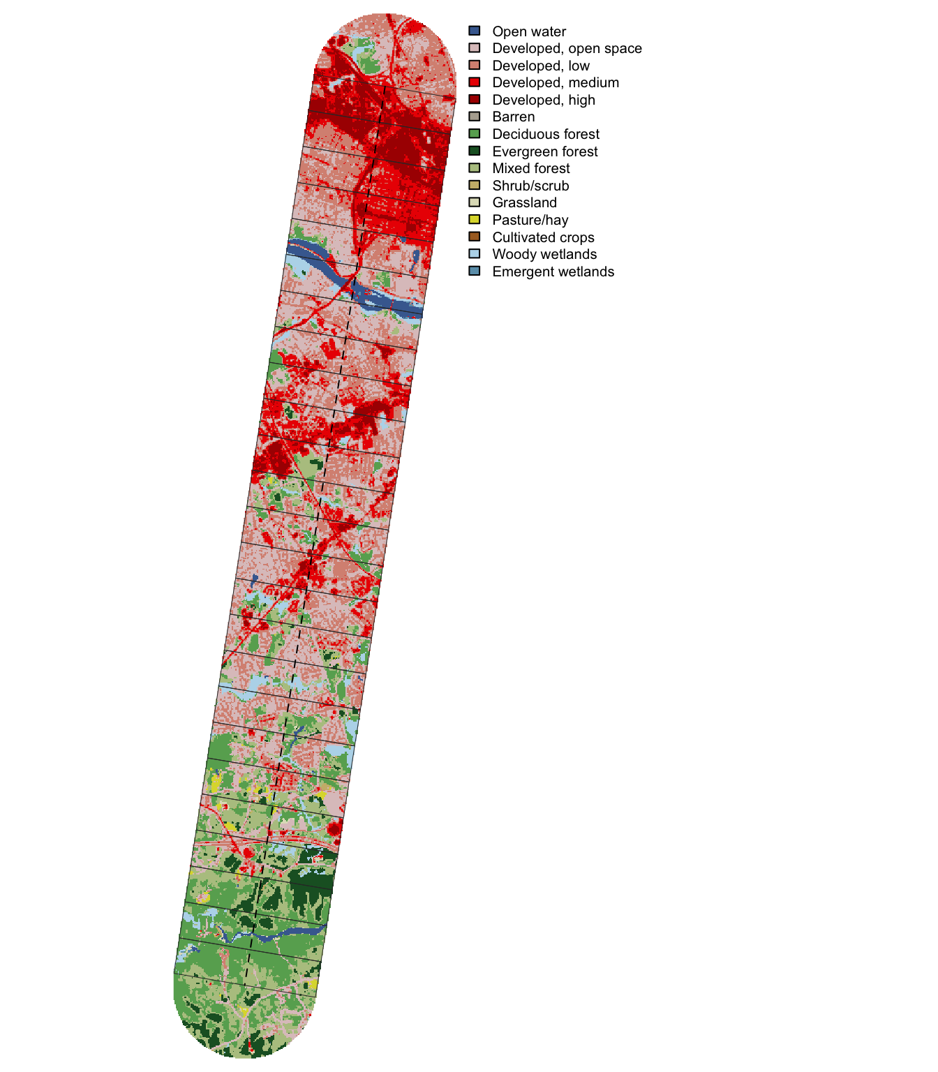
Annual NLCD land cover, impervious surface, and leaf-off NDVI along the transect
Published
November 4, 2026
Code
library(sf)library(dplyr)library(tidyr)library(ggplot2)library(leaflet)library(terra)library(here)source(here("R", "functions.R"))derived <-here(cfg$paths$derived)line <-load_transect()aoi <-load_aoi()windows <-load_windows()nlcd <-read.csv(file.path(derived, "nlcd_windows.csv"))classes <-read.csv(file.path(derived, "nlcd_window_classes.csv"))lc <-rast(here(cfg$nlcd$dir, sprintf("LndCov_%d.tif", cfg$nlcd$year)))ndvi_path <-file.path(derived, "ndvi_windows.csv")ndvi <-if (file.exists(ndvi_path)) read.csv(ndvi_path) elseNULL# Join on the window id only; the distance columns are floats and may not match exactlywindows <-left_join(windows, select(nlcd, -u_start_km, -u_end_km, -u_mid_km, -area_km2), by ="window")if (!is.null(ndvi)) windows <-left_join(windows, select(ndvi, -u_mid_km), by ="window")# Grouped cover, ordered from most to least urban; colors follow the NLCD legendcover_cols <-c(developed ="#eb0000",developed_open ="#dec5c5",barren ="#b3ac9f",agriculture ="#dcd939",shrub_grass ="#ccb879",forest ="#38814e",wetland ="#b8d9eb",water ="#466b9f")cover_labels <-c(developed ="Developed (low to high)", developed_open ="Developed, open space",barren ="Barren", agriculture ="Agriculture", shrub_grass ="Shrub and grassland",forest ="Forest", wetland ="Wetland", water ="Water")
Purpose
A first look at how land use changes from downtown Richmond to Pocahontas State Park. The study area is cut into non-overlapping 1 km windows along the transect, each spanning the full 4 km buffer width, and each window is summarized from the Annual NLCD 2025 land cover and fractional impervious surface layers (30 m) and from NDVI computed from the 4-band (RGB + near-infrared) 12-inch imagery.
NLCD is kept on its native grid (EPSG:5070). Windows are projected to it and summarized with exactextractr, which weights each 30 m cell by the fraction of it inside the window.
Windows
Code
n_win <-nrow(windows)
Windows: 25, each 1 km long by 4 km wide (the last is 0.99 km)
Area covered: 99.9 of 112.5 km². The round end caps beyond the endpoints are not part of any window.
Window 1 is at the Richmond end. Distance along the transect (u, km) is measured from the Richmond endpoint; transect_position() in R/functions.R returns u, the signed lateral offset v, and the window id for any point.
Use the layer control (top right) to choose which value colors the windows; hover a window for all of its values.
Code
to_ll <-function(x) st_transform(x, 4326)win_ll <-to_ll(windows)win_ll$label <-sprintf("<b>Window %d</b> (%.0f–%.0f km)<br>Impervious: %.1f%%<br>Developed: %.1f%%<br> Developed, open: %.1f%%<br>Forest: %.1f%%<br>Wetland + water: %.1f%%", win_ll$window, win_ll$u_start_km, win_ll$u_end_km, win_ll$imperv_mean, win_ll$developed_pct, win_ll$developed_open_pct, win_ll$forest_pct, win_ll$wetland_pct + win_ll$water_pct)win_ll$wet_water <- win_ll$wetland_pct + win_ll$water_pctif (!is.null(ndvi)) { win_ll$label <-paste0(win_ll$label, sprintf("<br>Evergreen (NDVI): %.1f%%", win_ll$evg_pct))}# One single-hue sequential scale per metric, all on a shared 0-100% domainmetrics <-list("Impervious surface"=list(col ="imperv_mean", pal ="Purples"),"Developed"=list(col ="developed_pct", pal ="Reds"),"Forest"=list(col ="forest_pct", pal ="Greens"),"Wetland + water"=list(col ="wet_water", pal ="Blues"))if (!is.null(ndvi)) metrics[["Evergreen (NDVI)"]] <-list(col ="evg_pct", pal ="BuGn")m <-leaflet(win_ll) |>addProviderTiles(providers$Esri.WorldGrayCanvas) |>addProviderTiles(providers$Esri.WorldImagery, group ="Imagery")for (nm innames(metrics)) { pal <-colorNumeric(metrics[[nm]]$pal, domain =c(0, 100)) m <- m |>addPolygons(color ="white", weight =1, fillOpacity =0.7,fillColor =pal(win_ll[[metrics[[nm]]$col]]),label =lapply(win_ll$label, htmltools::HTML),highlightOptions =highlightOptions(color ="black", weight =2, bringToFront =TRUE),group = nm) |>addLegend(pal = pal, values =c(0, 100), title =paste(nm, "(%)"),position ="bottomright", className ="info legend metric-legend",layerId = nm)}m |>addPolylines(data =to_ll(line), color ="black", dashArray ="6", weight =2) |>addLayersControl(baseGroups =names(metrics), overlayGroups ="Imagery",options =layersControlOptions(collapsed =FALSE)) |>hideGroup("Imagery") |># Leaflet does not hide legends for radio (base) layers; show only the selected metric's htmlwidgets::onRender(sprintf(" function(el, x) { var map = this; function show(name) { el.querySelectorAll('.metric-legend').forEach(function(lg) { lg.style.display = lg.textContent.trim().startsWith(name + ' (%%)') ? '' : 'none'; }); } show(%s); map.on('baselayerchange', function(e) { show(e.name); }); }", jsonlite::toJSON(names(metrics)[1], auto_unbox =TRUE)))
The charts below are interactive: hover to read every value at one distance, click a legend entry to hide it (double-click to show it alone), and drag to zoom (double-click to reset). Lines connect window midpoints, so values between midpoints are interpolated.
Code
library(plotly)# Shared x axis and landmarksriver_km <- nlcd$u_mid_km[which.max(nlcd$water_pct)]end_km <-max(nlcd$u_end_km)x_axis <-list(title ="Distance from Richmond (km)", range =c(0, end_km),dtick =5, zeroline =FALSE, showgrid =FALSE)landmarks <-list(list(x =0, y =1.02, yref ="paper", text ="Richmond", showarrow =FALSE,xanchor ="left", yanchor ="bottom", font =list(size =12)),list(x = end_km, y =1.02, yref ="paper", text ="Pocahontas State Park", showarrow =FALSE,xanchor ="right", yanchor ="bottom", font =list(size =12)),list(x = river_km, y =1.02, yref ="paper", text ="James River", showarrow =FALSE,yanchor ="bottom", font =list(size =12, color ="#466b9f")))river_line <-list(type ="line", x0 = river_km, x1 = river_km, y0 =0, y1 =1,yref ="paper", line =list(color ="#466b9f", width =1, dash ="dot"))plotly_cfg <-function(p) {config(p, displaylogo =FALSE,modeBarButtonsToRemove =c("lasso2d", "select2d", "autoScale2d"))}
Land cover composition
Share of each window in each grouped cover type. Developed land is stacked from the bottom and forest above it, so the urban-to-forest transition reads as the green band widening toward Pocahontas State Park.
Code
p <-plot_ly()for (k innames(cover_cols)) { p <-add_trace(p, data = nlcd, x =~u_mid_km, y = nlcd[[paste0(k, "_pct")]],type ="scatter", mode ="lines", stackgroup ="cover",name = cover_labels[[k]], fillcolor = cover_cols[[k]],line =list(color ="white", width =0.5),hovertemplate =paste0(cover_labels[[k]], ": %{y:.1f}%<extra></extra>"))}p |>layout(xaxis =c(x_axis, list(hoverformat =".1f")),yaxis =list(title ="Share of window (%)", range =c(0, 100), ticksuffix ="%"),hovermode ="x unified",legend =list(traceorder ="reversed"),annotations = landmarks, shapes =list(river_line),margin =list(t =40)) |>plotly_cfg()
Impervious surface and forest
Mean fractional impervious surface and forest cover per window. The shaded band is ± 1 SD of impervious surface among the 30 m cells in each window, a measure of how mixed the window is.
cat(sprintf("The imagery was flown leaf-off, so near-infrared greenness mostly marks evergreen foliage(pine, cedar, holly, magnolia, evergreen shrubs) and green winter lawns. *Evergreen* is theshare of 1 ft pixels in a window with brightness-adjusted NDVI above %s, the same thresholdused to measure evergreen surroundings for holly candidates (plain NDVI is inflated in shadow;see the [holly page](03_holly_classification.qmd#shadows)); open water is excluded. The forest-only lineuses the same measure within NLCD forest (classes 41–43) and reads as the evergreenshare of the forest canopy. NLCD forest cover is shown for reference.",cfg$holly$thresholds$ndvi_adj$context))
The imagery was flown leaf-off, so near-infrared greenness mostly marks evergreen foliage (pine, cedar, holly, magnolia, evergreen shrubs) and green winter lawns. Evergreen is the share of 1 ft pixels in a window with brightness-adjusted NDVI above 1, the same threshold used to measure evergreen surroundings for holly candidates (plain NDVI is inflated in shadow; see the holly page); open water is excluded. The forest-only line uses the same measure within NLCD forest (classes 41–43) and reads as the evergreen share of the forest canopy. NLCD forest cover is shown for reference.
Code
nd <-left_join(ndvi, select(nlcd, window, forest_pct), by ="window")evg_col <-"#01665e"plot_ly(nd, x =~u_mid_km) |>add_trace(y =~evg_pct, type ="scatter", mode ="lines+markers", name ="Evergreen, all land",line =list(color = evg_col, width =2), marker =list(color = evg_col, size =8),hovertemplate ="Evergreen, all land: %{y:.1f}%<extra></extra>") |>add_trace(y =~evg_forest_pct, type ="scatter", mode ="lines+markers",name ="Evergreen, within forest",line =list(color = evg_col, width =2, dash ="dash"),marker =list(color = evg_col, size =8, symbol ="circle-open"),hovertemplate ="Evergreen, within forest: %{y:.1f}%<extra></extra>") |>add_trace(y =~forest_pct, type ="scatter", mode ="lines", name ="NLCD forest cover",line =list(color ="#38814e", width =1.5, dash ="dot"),hovertemplate ="NLCD forest: %{y:.1f}%<extra></extra>") |>layout(xaxis =c(x_axis, list(hoverformat =".1f")),yaxis =list(title ="Percent", range =c(0, 100), ticksuffix ="%"),hovermode ="x unified",legend =list(orientation ="h", y =-0.2),annotations = landmarks, shapes =list(river_line),margin =list(t =40)) |>plotly_cfg()
Evergreen cover follows the urban-to-forest gradient only loosely. It is lowest in downtown Richmond (about 7–9% at km 0–2), sits between about 12% and 22% through most of the transect, and peaks at 43% at km 21–22, where pine stands are common. In the developed windows part of the signal is green winter lawn and street trees rather than evergreen canopy; the adjusted index is calibrated on forest, so it is least reliable on bright urban surfaces.
Within forest the evergreen share does not follow the urban gradient. The small forest patches near km 9–11 are pine-rich (41–46% evergreen), the forests at km 12–20 are mostly deciduous (18–28%), km 21–22 is pine-rich again (54%), and km 23–24 is hardwood-dominated (about 19%). The amount of forest (NLCD) and its composition (NDVI) change at different places along the transect. That matters for holly: an isolated evergreen crown is easiest to see, and most likely to be holly, in deciduous forest. Windows 1–4 have no NLCD forest, so they have no forest-only value.
Data: Annual NLCD Collection 1, 2025 land cover (LndCov) and fractional impervious surface (FctImp), read for the AOI bounding box from the USGS web coverage service (https://dmsdata.cr.usgs.gov/geoserver). No resampling or reprojection of the rasters.
Developed combines NLCD classes 22–24 (low, medium, high intensity). Developed open space (21) is mostly lawns, parks, and road verges and is kept separate. Forest is classes 41–43; wetland is 90 and 95.
NDVI: computed at full 1 ft resolution from the 4-band VBMP tiles and summarized into 10 ft cells (mean NDVI and share of pixels above the evergreen threshold) before the window summaries. NLCD is resampled to the 10 ft grid (nearest neighbour) only to mask water and select forest. The NIR band is not radiometrically calibrated, so NDVI values are relative to this imagery, and leaf-off timing means NDVI says little about deciduous canopy.
Windows are not replicated samples. Adjacent windows are spatially autocorrelated, so the curves describe the gradient but should not be treated as 25 independent observations.
The 4 km width averages across very different ground on either side of the line (e.g. the James River crossing near 5–7 km). A narrower center band would test how much that matters.