Forest Composition

Evergreen and deciduous shares of NLCD forest from leaf-off imagery

library(dplyr)
library(tidyr)
library(ggplot2)
library(plotly)
library(here)

source(here("R", "functions.R"))
derived <- here(cfg$paths$derived)
fcfg <- cfg$forest_composition

pts  <- read.csv(file.path(derived, "forest_points.csv"))
mix  <- read.csv(file.path(derived, "forest_mixture.csv"))
comp <- read.csv(file.path(derived, "forest_composition.csv"))
cls  <- read.csv(file.path(derived, "nlcd_window_classes.csv"))

cls_est <- comp[grepl("^nlcd_", comp$group), ]
cls_est$nlcd <- as.integer(sub("nlcd_", "", cls_est$group))
win_est <- comp[!is.na(comp$window) & comp$n >= 30, ]
tot <- comp[comp$group == "windows_total", ]
pct <- function(x, d = 0) sprintf(paste0("%.", d, "f%%"), 100 * x)
crown_thr <- cfg$holly$thresholds$ndvi_adj$crown

Purpose

NLCD splits forest into deciduous (41), evergreen (42), and mixed (43), but only at 30 m and from classified Landsat. The leaf-off orthoimagery shows evergreen foliage directly, at 1 ft. This page uses it to estimate what share of NLCD forest is evergreen and what share is deciduous, for each forest class and for each 1 km window along the transect.

Across the windows, NLCD maps 24.8 km² of forest. Of that, an estimated 29% is evergreen (95% interval 27%–31%), about 7.2 km², and 17.6 km² is deciduous.

Step	Script	Output
11. Forest sample, mixture, shares	R/09_forest_composition.R	data/derived/forest_points.csv, forest_mixture.csv, forest_composition.csv

Method

Sample. 48,517 random points in NLCD forest, at the same density everywhere (about 6000 in the most forested window). Each point gets its brightness-adjusted NDVI (ndvi_adj, see Holly candidates), averaged over its 3 × 3 ft neighbourhood. On this scale bare hardwood is near 0 at any brightness and evergreen foliage is higher.

Why not a threshold. The two kinds of pixel overlap. A cutoff that keeps false positives low misses most evergreen, and one that catches most evergreen also passes many deciduous pixels. In both cases the error depends on the true mix. For example, only 31% of points in NLCD evergreen forest exceed the crown threshold (1.7).

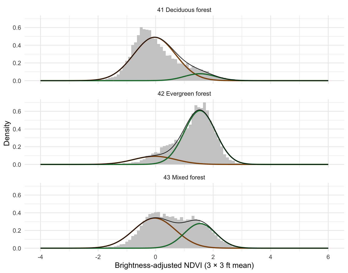
Mixture model. Instead, a two-component Gaussian mixture is fitted to all forest points pooled: one deciduous component and one evergreen component. The two components are then held fixed, and only the evergreen weight is re-estimated for each NLCD class and each window. That weight is the estimated share of forest area whose visible winter foliage is evergreen. The intervals come from 200 bootstrap replicates, each resampling points within windows and refitting the mixture, so they include uncertainty in the components themselves.

mix |>
  transmute(Component = component, `Mean ndvi_adj` = round(mean, 2),
            `95% interval of mean` = sprintf("%.2f to %.2f", mean_lo, mean_hi),
            SD = round(sd, 2), `Weight (all forest)` = pct(weight, 1)) |>
  knitr::kable()

Component	Mean ndvi_adj	95% interval of mean	SD	Weight (all forest)
deciduous	-0.04	-0.07 to -0.01	0.73	69.4%
evergreen	1.54	1.51 to 1.57	0.55	30.6%

lab <- c(`41` = "41 Deciduous forest", `42` = "42 Evergreen forest", `43` = "43 Mixed forest")
p <- pts |> filter(ndvi_adj > -4, ndvi_adj < 6)
xs <- seq(-4, 6, by = 0.02)
dens <- cls_est |>
  rowwise() |>
  reframe(nlcd = nlcd, x = xs,
          deciduous = (1 - evg_share) * dnorm(xs, mix$mean[1], mix$sd[1]),
          evergreen = evg_share * dnorm(xs, mix$mean[2], mix$sd[2])) |>
  mutate(total = deciduous + evergreen)
ggplot(p, aes(ndvi_adj)) +
  geom_histogram(aes(y = after_stat(density)), binwidth = 0.1, fill = "grey80") +
  geom_line(data = dens, aes(x, deciduous), colour = "#8c510a", linewidth = 0.8) +
  geom_line(data = dens, aes(x, evergreen), colour = "#1b7837", linewidth = 0.8) +
  geom_line(data = dens, aes(x, total), linewidth = 0.4) +
  facet_wrap(~nlcd, ncol = 1, labeller = as_labeller(lab)) +
  labs(x = "Brightness-adjusted NDVI (3 × 3 ft mean)", y = "Density") +
  theme_minimal()

ndvi_adj of forest points by NLCD class (histograms), with the fitted deciduous (brown) and evergreen (green) components scaled by each class’s estimated weights. The black line is their sum.

Check against NLCD

NLCD defines its forest classes by the share of trees that keep their leaves all year: deciduous forest under 25% evergreen, evergreen forest over 75%, and mixed forest in between. The image-based estimates, made without using those labels, fall in the same ranges:

cls_est |>
  mutate(Class = lab[as.character(nlcd)],
         `NLCD definition` = c("< 25% evergreen", "> 75% evergreen", "25–75% evergreen"),
         `Estimated evergreen` = sprintf("%s (%s–%s)", pct(evg_share, 1), pct(lo, 1), pct(hi, 1)),
         `Points above crown threshold` = pct(share_gt_crown, 1)) |>
  select(Class, Points = n, `NLCD definition`, `Estimated evergreen`,
         `Points above crown threshold`) |>
  knitr::kable(format.args = list(big.mark = ","))

	Class	Points	NLCD definition	Estimated evergreen	Points above crown threshold
2	41 Deciduous forest	22,265	< 25% evergreen	10.7% (9.3%–12.2%)	5.5%
3	42 Evergreen forest	6,307	> 75% evergreen	83.2% (81.3%–85.2%)	30.6%
4	43 Mixed forest	19,945	25–75% evergreen	38.1% (36.0%–40.7%)	13.6%

The last column shows how far a simple threshold would be off.

Along the gradient

nlcd_proxy <- cls |>
  filter(class %in% 41:43) |>
  group_by(window) |>
  summarise(proxy = sum(frac * c(`41` = 0, `42` = 1, `43` = 0.5)[as.character(class)]) / sum(frac),
            .groups = "drop")
g <- win_est |>
  left_join(nlcd_proxy, by = "window") |>
  mutate(km = sprintf("%g–%g", u_mid_km - 0.5, u_mid_km + 0.5))

plot_ly(g, x = ~u_mid_km) |>
  add_bars(y = ~evg_km2, name = "Evergreen", marker = list(color = "#1b7837"),
           text = ~sprintf("km %s<br>Evergreen %.2f km² (%s)", km, evg_km2, pct(evg_share)),
           hoverinfo = "text", textposition = "none") |>
  add_bars(y = ~dec_km2, name = "Deciduous", marker = list(color = "#bf812d"),
           text = ~sprintf("km %s<br>Deciduous %.2f km²", km, dec_km2),
           hoverinfo = "text", textposition = "none") |>
  layout(barmode = "stack", bargap = 0.1,
         xaxis = list(title = "Distance from Richmond (km)"),
         yaxis = list(title = "NLCD forest area in window (km²)"),
         legend = list(orientation = "h", y = 1.1))

plot_ly(g, x = ~u_mid_km) |>
  add_ribbons(ymin = ~100 * lo, ymax = ~100 * hi, name = "95% interval",
              fillcolor = "rgba(27,120,55,0.2)", line = list(width = 0), hoverinfo = "none") |>
  add_lines(y = ~100 * evg_share, name = "Evergreen share (imagery)",
            line = list(color = "#1b7837", width = 2),
            text = ~sprintf("km %s<br>%s (%s–%s), %d points", km, pct(evg_share), pct(lo),
                            pct(hi), n), hoverinfo = "text") |>
  add_lines(y = ~100 * proxy, name = "NLCD labels (42 = 100%, 43 = 50%)",
            line = list(color = "grey40", dash = "dot"),
            text = ~sprintf("km %s<br>NLCD-label proxy %s", km, pct(proxy)), hoverinfo = "text") |>
  layout(xaxis = list(title = "Distance from Richmond (km)"),
         yaxis = list(title = "Evergreen share of forest (%)", rangemode = "tozero"),
         hovermode = "x unified", legend = list(orientation = "h", y = 1.1))

Windows with no NLCD forest (km 0–4, downtown and the James River) have no estimate. Evergreen share is highest at km 21–22 (62%) and km 10–11 (58%); pine stands are the likely cause, but this has not been checked on the ground. Elsewhere south of km 14 the forest is 13%–39% evergreen. The windows nearest the city (km 4–9) have little forest, and it is mostly deciduous (6%–22% evergreen). The imagery estimate follows the NLCD-label proxy closely (r = 0.80 across windows), but the proxy treats every mixed-forest cell as half evergreen and every deciduous cell as none.

g |>
  transmute(Window = window, km, Points = n,
            `Forest (km²)` = round(forest_km2, 2),
            `Evergreen` = sprintf("%s (%s–%s)", pct(evg_share), pct(lo), pct(hi)),
            `Evergreen (km²)` = round(evg_km2, 2), `Deciduous (km²)` = round(dec_km2, 2),
            `NLCD-label proxy` = pct(proxy)) |>
  knitr::kable()

Window	km	Points	Forest (km²)	Evergreen	Evergreen (km²)	Deciduous (km²)	NLCD-label proxy
5	4–5	413	0.26	16% (11%–20%)	0.04	0.22	15%
6	5–6	362	0.22	6% (2%–9%)	0.01	0.21	21%
7	6–7	333	0.23	11% (5%–15%)	0.02	0.20	31%
8	7–8	261	0.16	11% (5%–17%)	0.02	0.14	11%
9	8–9	265	0.17	22% (15%–30%)	0.04	0.13	8%
10	9–10	149	0.10	43% (34%–53%)	0.04	0.06	65%
11	10–11	731	0.51	58% (53%–63%)	0.29	0.21	47%
12	11–12	1381	0.91	27% (24%–32%)	0.25	0.66	35%
13	12–13	707	0.45	19% (15%–23%)	0.09	0.37	7%
14	13–14	269	0.17	24% (17%–30%)	0.04	0.13	7%
15	14–15	1087	0.63	28% (24%–32%)	0.17	0.45	27%
16	15–16	1418	0.92	24% (21%–27%)	0.22	0.70	29%
17	16–17	1287	0.84	19% (16%–22%)	0.16	0.68	23%
18	17–18	1550	0.98	21% (18%–25%)	0.21	0.77	28%
19	18–19	2386	1.50	13% (11%–15%)	0.19	1.31	18%
20	19–20	2823	1.76	25% (22%–28%)	0.44	1.32	30%
21	20–21	3298	2.06	34% (31%–37%)	0.70	1.36	38%
22	21–22	3931	2.51	62% (60%–64%)	1.57	0.95	63%
23	22–23	6041	3.78	39% (36%–41%)	1.46	2.32	45%
24	23–24	5206	3.25	13% (11%–16%)	0.44	2.81	17%
25	23.9932–24.9932	5474	3.43	23% (21%–25%)	0.80	2.63	21%

Notes

• Leaf-off means “visible evergreen”. In winter, evergreen understory (holly, cedar, mountain laurel, evergreen shrubs) shows through bare hardwood canopy and counts as evergreen. These shares are therefore the evergreen part of what is seen from above in winter, and can be higher than the evergreen share of the leaf-on canopy. For holly this is useful: understory evergreens are part of what holly lives among.
• Fixed components. The method assumes deciduous and evergreen pixels have the same ndvi_adj distribution everywhere. Differences in flight date, sun angle, or species mix along the transect would shift the components and bias some windows. The class check above suggests this is not a large effect overall, but it is not tested window by window.
• NLCD forest boundaries. Forest is defined by the 30 m NLCD map, so the sample includes some gaps, edges, and roads inside forest cells, and leaves out trees outside mapped forest (street trees, yards). Those count toward neither share.
• Small samples near the city. Windows with little forest have few points and wide intervals.
• Not species. “Evergreen” lumps pine, cedar, holly, and evergreen shrubs; separating them would need texture or crown shape, or a leaf-on image to compare against.