Plotting Points
Simply having a bunch of points is not enough. We gotta see it! Here are some examples to get you started.
The Data
Here we will use the enigmatic Araptus attenuata data set as a raw data.frame
##       Site      Longitude         Latitude         Males
##  12     : 1   Min.   :-114.3   Min.   :23.29   Min.   : 9.00
##  153    : 1   1st Qu.:-113.2   1st Qu.:24.88   1st Qu.:16.00
##  157    : 1   Median :-112.0   Median :26.64   Median :19.00
##  159    : 1   Mean   :-111.9   Mean   :26.42   Mean   :24.93
##  160    : 1   3rd Qu.:-110.7   3rd Qu.:28.04   3rd Qu.:28.00
##  161    : 1   Max.   :-109.3   Max.   :29.33   Max.   :64.00
##  (Other):23
##     Females       Suitability
##  Min.   : 5.00   Min.   :0.05628
##  1st Qu.:15.00   1st Qu.:0.26730
##  Median :21.00   Median :0.41251
##  Mean   :23.62   Mean   :0.43527
##  3rd Qu.:30.00   3rd Qu.:0.56413
##  Max.   :63.00   Max.   :0.90188
##
and as a sf object
library(sf)
araptus_sf <- st_as_sf(araptus,coords = c("Longitude","Latitude"))
st_crs(araptus_sf) <- 3857
araptus_sf
## Simple feature collection with 29 features and 4 fields
## geometry type: POINT
## dimension: XY
## bbox: xmin: -114.2935 ymin: 23.2855 xmax: -109.327 ymax: 29.32541
## epsg (SRID): 3857
## proj4string: +proj=merc +a=6378137 +b=6378137 +lat_ts=0.0 +lon_0=0.0 +x_0=0.0 +y_0=0 +k=1.0 +units=m +nadgrids=@null +wktext +no_defs
## First 10 features:
## Site Males Females Suitability geometry
## 1 12 24 21 0.3519050 POINT (-112.6655 27.18232)
## 2 153 35 41 0.7324870 POINT (-110.4624 24.13389)
## 3 157 26 30 0.8810290 POINT (-110.096 24.0195)
## 4 159 22 15 0.1879650 POINT (-113.3161 27.52944)
## 5 160 48 36 0.3651910 POINT (-112.5296 27.40498)
## 6 161 64 63 0.2791050 POINT (-112.986 27.0367)
## 7 162 57 41 0.6136198 POINT (-112.408 27.2028)
## 8 163 21 21 0.4328730 POINT (-110.951 24.2115)
## 9 166 19 26 0.2673030 POINT (-112.0806 25.91409)
## 10 168 28 25 0.4964650 POINT (-111.2156 25.55757)See point construction for a discussion on the differences between data.frame and sf objects.
Plotting data.frame Points
A set of points is useful in some context. Here is how we can plot these points using the normal ggplot routines. The background map_data is an extension of the ggplot library to grab map sections. Here is the polygon for Mexico.
library(ggplot2)
library(dplyr)
library(DT)
map_data("world") %>%
  filter( region == "Mexico", is.na(subregion)) -> baja
datatable( baja )
which as you can see is a dataframe of points to be connected into a single object. We can plot it using normal approaches as:
ggplot() +
  geom_polygon( aes(long,lat), fill="grey", data=baja ) +
  geom_point( aes(Longitude,Latitude), data=araptus ) +
  xlab("Longitude") +
  ylab("Latitude") +
  coord_map()
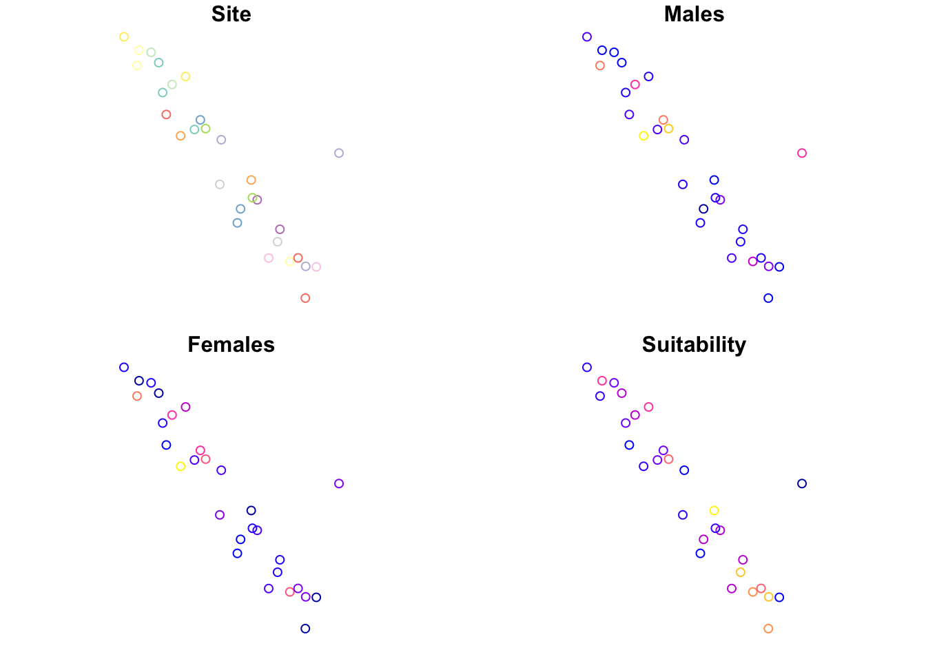
Plotting sf Objects
The sf library also has a bunch of built-in plotting routines. If you plot a sf object, it will make a plot for each of the columns of the data in the object. For example, the araptus_sf object has the following data associated with each point
## [1] "Site" "Males" "Females" "Suitability" "geometry"and as such will plot one graph for each column.
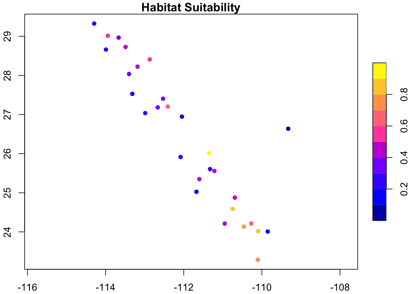
You can specify a single plot as (and set default values:
It is also possible to plot sf objects using ggplot as they supply appropriate geom_ and coord_ objects.
ggplot() +
  geom_sf( data = araptus_sf, aes(size=Suitability) )  +
  theme_void() +
  coord_sf( datum=NA )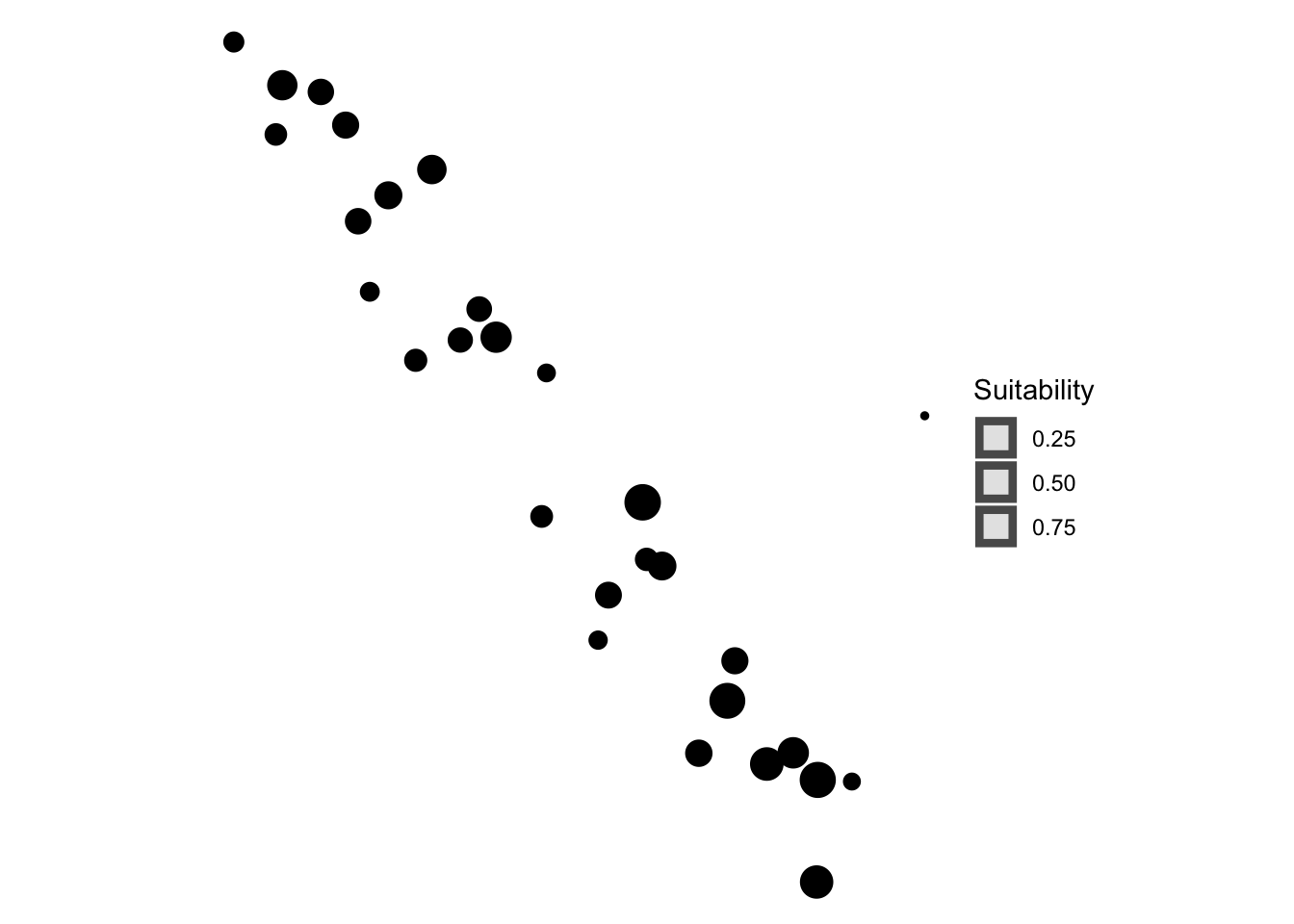
Interactive Maps
Since this document is in HTML, we can take advantage of interactive visualizations. This is a good thing ©. Here is an interactive leaflet map with each sampling locale designated by a circle whose radius is proportional to the habitat suitability of the host plant, all plot on the ESRI World Topo map.
library(leaflet)
leaflet(araptus) %>%
  addProviderTiles( providers$Esri.WorldTopoMap) %>%
  addCircleMarkers( radius = ~Suitability*10, color="green",label = ~Site)
We can even get a bit more fancy in making pie charts representing the numbrer of males and females in each population, scaled by the habitat suitability.