Projections

Impetus

Our ability to use and understand spatial data is dependent upon understanding geographic ellipses, coordinate systems, and datum. A spatial projection is a mathematical representation of a coordinate space used to identify geospatial objects. Because the earth is both non-flat and non-spheroid, we must use mathematical approaches to describe the shape of the earth in a coordinate space. We do this using an ellipsoid—a simplified model of the shape of the earth.

Basics

To define an ellipsoid, it is necessary to define a mathematica model of the earth. These models can come in a wide variety of forms, but common ones include:

• NAD27 (North American Datum of 1927) based upon land surveys
  
• NAD83 based upon satellite data measuring the distance of the surface of the earth to the center of the plant. This is also internationally known as GRS80 (Geodetic Reference System 1980) internationally.
  
• WGS84 (World Geodetic System 1984) is a refinement of GRS80 done by the US military that was used in the development of GPS systems (and subsequently for all of us).

A projection onto an ellipsoid is a way of converting the spherical coordinates, such as longitude and latitude, into 2-dimensional coordinates we can use. There are three main types of approaches that have been used to develop various projections. (see wikipedia for some example imagery of different projections).

These include:

• Azimuthal: An approach in which each region of the earth is projected onto a plane tangential to the surface, typically at the pole or equator.
  
• Cylindrical: This approach projects the surface of the earth onto a cylinder, which is ‘unrolled’ like a large map. This approach ‘stretches’ distances in a east-west fashion, which is why Greenland looks so large…
• Conic: Another ‘unrolling’ approach, though this time instead of a cylinder, it is projected onto a cone.

All projections produce bias in area, distance, or shape (some do so in more than one), so there is no ‘optimal’ projection. To give you an idea of the consequences of these projections, I’ll use the United States map as an example and we can visualize how it is projected onto a 2-dimensional space using different projections.

Equatorial Projections

These are projections centered on the Prime Meridian (Longitude=0)

library(maps)
par(mfrow=c(2,2), mar=c(0,0,0,0)) # makes 2x2 grid of images with no margin
map("state",proj="mercator",main="mercator")
map("state",proj="mollweide", main="mollweide")
map("state",proj="gilbert", main="gilbert")
map("state",proj="cylequalarea",par=39.83)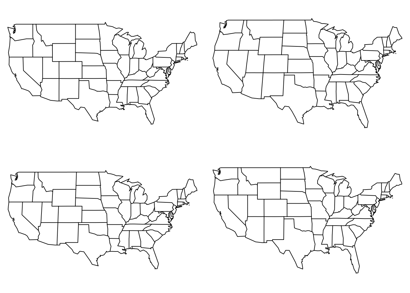

Mercator, Mollweide, and Gilbert equatorial projections along with a cylequalarea projection centered on the middle of the US.

Azimuth Projections

These projections are centered on the North Pole with parallels making concentric circles. Meridians are equally spaced radial lines.

par(mfrow=c(2,2), mar=c(0,0,0,0))
map("state",proj="orthographic")
map("state",proj="orthographic")
map("state",proj="perspective", param=8)
map("state",proj="gnomonic")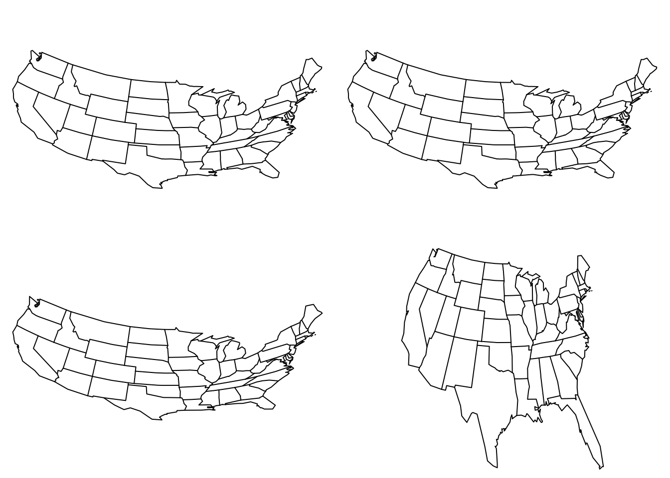

Orthographic, stereographic, perspective, and gnomonic projections.

Polar Conic Projections

Here projections are symmetric around the Prime Meridian with parallel as segments of concentric circles with meridians being equally spaced.

par(mfrow=c(1,2), mar=c(0,0,0,0))
map("state",proj="conic",par=39.83)
map("state",proj="lambert",par=c(30,40))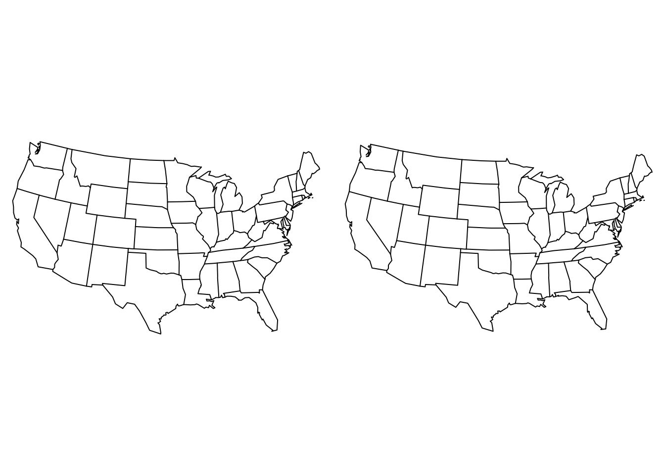

Conic and Lambert projections.

Miscellaneous Projections

These are some additional miscellaneous projections, provided for fun mostly, to show some more diversity in the ways we have come up with mapping points onto 2-dimensional displays.

par(mfrow=c(2,2), mar=c(0,0,0,0))
map("state",proj="square")
map("state",proj="hex")
map("state",proj="bicentric", par=-98)
map("state",proj="guyou")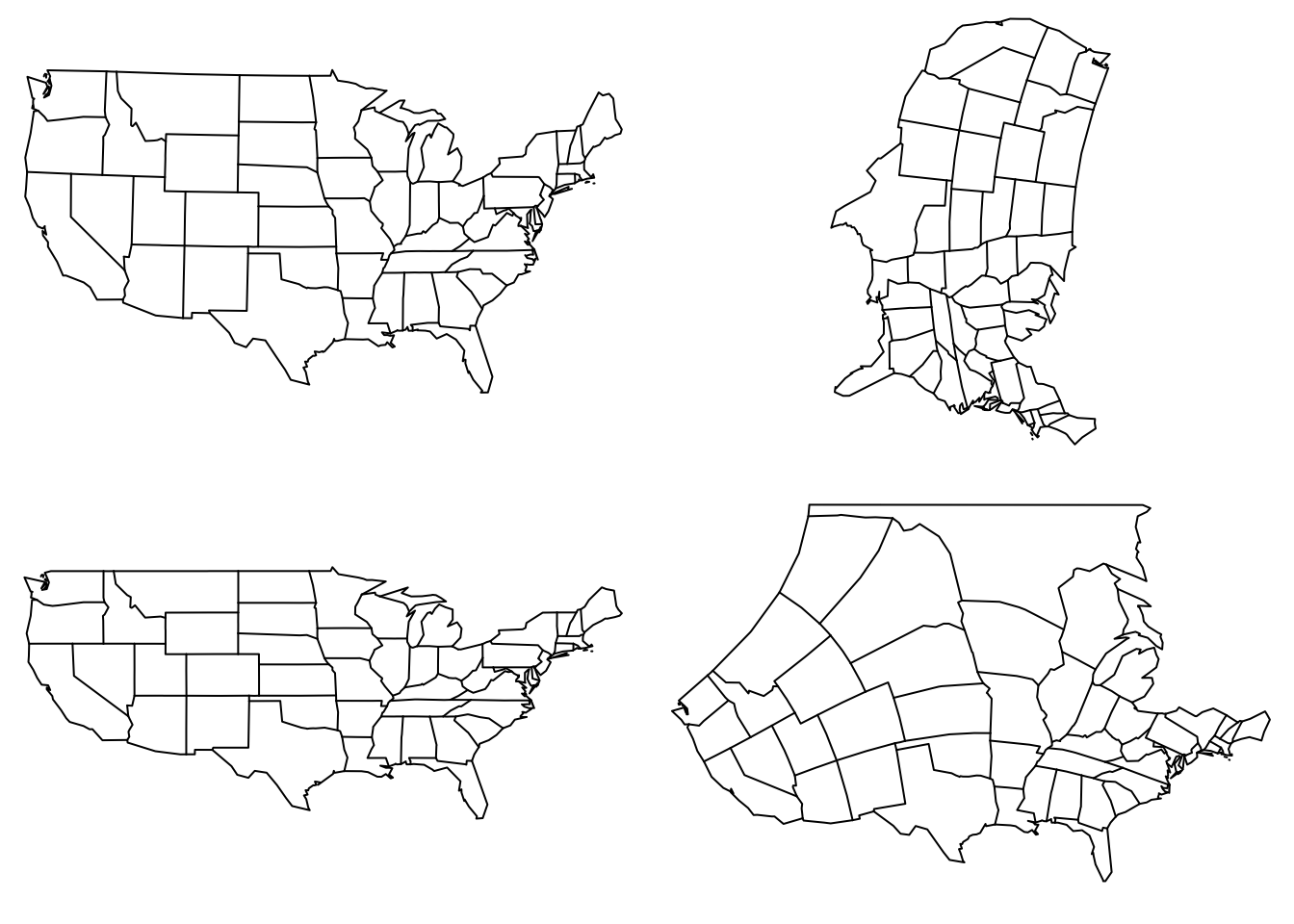

Miscellaneous projections (Square, hex, bicentric, and Guyou) highlighting some of the more excentric ways of displaying data.

ggplot2 Plotting

In addition to plotting routines from the map library, ggplot2 also includes the ability to define specific projections. Internally, the map object is just a data.frame.

us <- map_data("state")
summary(us)

##       long              lat            group           order      
##  Min.   :-124.68   Min.   :25.13   Min.   : 1.00   Min.   :    1  
##  1st Qu.: -96.22   1st Qu.:33.91   1st Qu.:15.00   1st Qu.: 3899  
##  Median : -87.61   Median :38.18   Median :26.00   Median : 7794  
##  Mean   : -89.67   Mean   :38.18   Mean   :30.15   Mean   : 7798  
##  3rd Qu.: -79.13   3rd Qu.:42.80   3rd Qu.:47.00   3rd Qu.:11699  
##  Max.   : -67.01   Max.   :49.38   Max.   :63.00   Max.   :15599  
##     region           subregion        
##  Length:15537       Length:15537      
##  Class :character   Class :character  
##  Mode  :character   Mode  :character  
##                                       
##                                       
## 

library(ggplot2)
us_map <- ggplot( us, aes(x=long, y = lat, group=group) ) + geom_polygon( fill="white", color="black")
us_map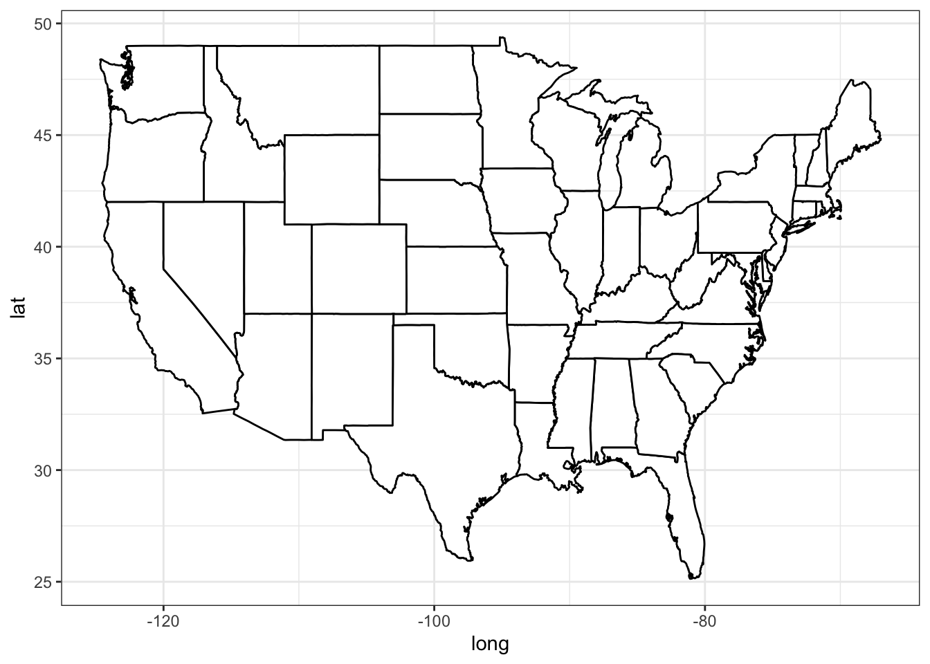

Application of a projeted coordinate system via coord_map produces the same output (whose default projection is mercator).

us_map + coord_map()

us_map + coord_map(projection="azequalarea")

us_map + coord_map( projection="guyou")

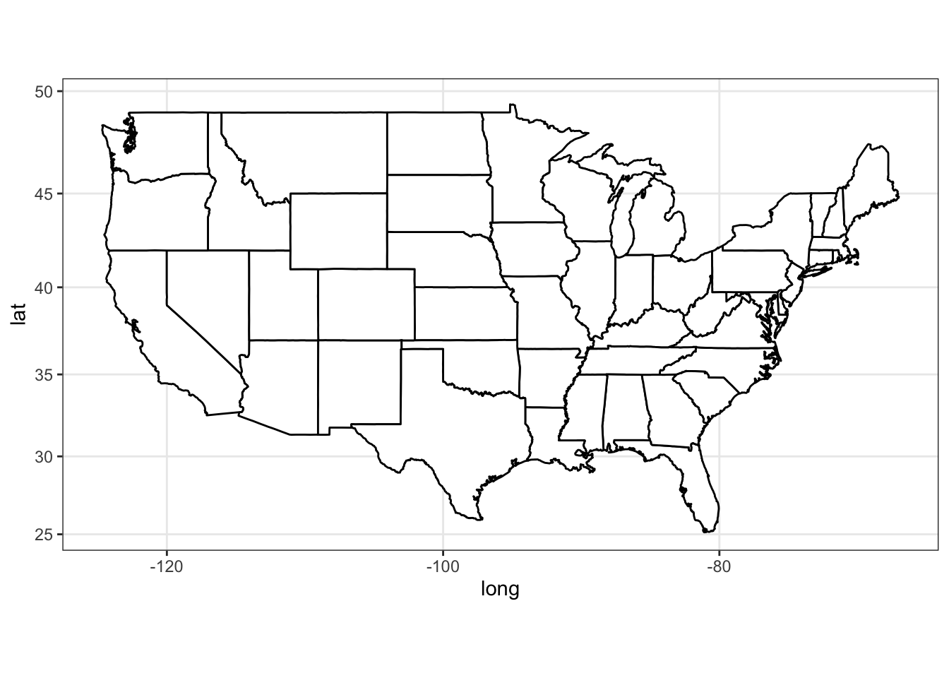
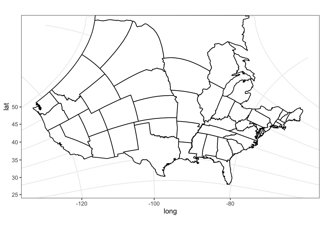
See ?coord_map for other a list of available projections.

Coordinate Systems

Onto this ellipsoid, we must define a set of reference locations (in 3-space) called datum that help describe the precise shape of the surface. We typically are dealing with a combination of data that we’ve collected and that we’ve attained from some other provider. In most GIS applications, the coordinate systems we encounter are either:

• UTM (Universal Transverse Mercator) measuring the distance from the prime meridian for the x-coordinate and the distance from the equator (often called northing in the northern hemisphere) for the y-coordinate. These distances are in meters and the globe is divided into 60 zones, each of which is 6 degrees in width. Geographic coordinate systems use longitude and latitude. For historical purposes these are unfortunately reported in degrees, minutes, seconds, a temporal abstraction that is both annoying and a waste of time (IMHO).
  
• Decimal degrees, while less easy to remember, are easier to work with in R.
• State Planar coordinate systems are coordinate systems that each US State has defined for their own purposes. They are based upon some arbitrarily defined points of reference and another pain to use (IMHO). Given the differential in state area, some states are also divided into different zones. Maps you get from municipal agencies may be in this coordinate system. If your study straddles different zones or even state lines, you have some work ahead of you…

It is best to use a system that is designed for your kind of work. Do not, for example, use a state plane system outside of that state as you have bias associated with the distance away from the origin. That said, Longitude/Latitude (decimal degrees) and UTM systems are probably the easiest to work with in R.

Projection Summary

It is in your best interest to get your data into a single and uniform projection, in the same coordinate system, with the same datum. Until you do that, you cannot really start working with your data. In the sections below, we show how to set these and reproject them for uniformity.