Visualizing Rasters

Visualizing data contained in a raster is a fundamental task that can be handled by many different conditions. For this example, we will use the Baja California elevation raster.

library(raster)
r <- raster("data/alt_22.tif")
baja_california <- crop(r, extent( c(-115,-109,22,30) ) )
baja_california

## class      : RasterLayer 
## dimensions : 960, 720, 691200  (nrow, ncol, ncell)
## resolution : 0.008333333, 0.008333333  (x, y)
## extent     : -115, -109, 22, 30  (xmin, xmax, ymin, ymax)
## crs        : +proj=longlat +datum=WGS84 +no_defs +ellps=WGS84 +towgs84=0,0,0 
## source     : /private/var/folders/ty/1tdv5mw56p33qx86hnk5h8l80000gn/T/Rtmp72DZ9d/raster/r_tmp_2019-11-21_150945_13287_99586.grd 
## names      : alt_22 
## values     : -202, 2263  (min, max)

Basic Plotting

As part of the built-in object, a raster has the following methods available.

methods(class="raster")

## [1] [         [<-       anyNA     as.matrix as.raster is.na     Ops      
## [8] plot      print    
## see '?methods' for accessing help and source code

of which the plot is the most relevant for this page.

plot(baja_california)

This is the normal plotting functions so we can fancy it up using the normal kind of options to the plot command:

plot( baja_california, 
      xlab = "Longitude", ylab = "Latitude",
      main = "Elevation for Baja California",
      col=terrain.colors(50) )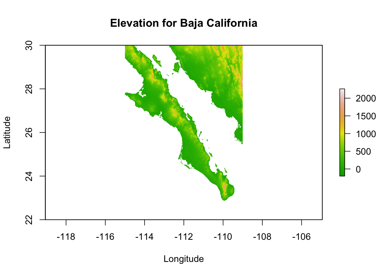

Rasters & ggplot

You can also use ggplot to plot your rasters using geom_tile.

library(ggplot2)
df <- data.frame( rasterToPoints( baja_california )) 
names(df) <- c("Longitude","Latitude","Elevation")
p <- ggplot( df ) + geom_tile( aes(x=Longitude,y=Latitude,fill=Elevation)) 
p <- p + scale_fill_gradientn( colors=c('#a6611a','#dfc27d','#f5f5f5','#80cdc1','#018571'))
p <- p + coord_equal() + xlab("Longitude") + ylab("Latitude") 
p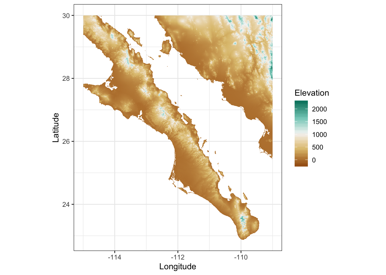

3-Dimensional Visualization

It is also possible to visualize rasters in 3-space. The library rasterVis provides an interface to the rgl library to plot a surface. Once installed, these are easy to use for viewing surfaces. Here is an example using the elevation data we have been playing with.

library(rasterVis)
plot3D( baja_california , zfac=0.1)

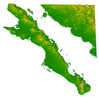
The zfac option in the plot is the amount to scale the z-axis (elevation) in relation to the x-axis and y-axis dimensions. It is a bit exaggerated at zfac=0.1 but you get the idea.

this is some new stuff