26 Linear Models

If you boil it down to the base essence of population genetic analyses, we can define almost all of our analyses by the following fundamental equation. Ultimately, a set of genetic data (\(G\)) is crated and we are attempting to describe patterns or variation in this data by fitting (via some function \(f()\)) to it one ore more independent variables (\(E\)).

\[ G = f(E) \]

These independent variables may be:

• Categorical: Populations, sex, habitat type, etc. This is the most common type of external variable addressed by thousands of hypotheses such as, \(H_O:F_{ST}=0\). More complicated examples may include hierarchical structure such as individuals nested within locales, locales contained within regions, etc.
• Continuous: Elevation, Latitude, Longitude, etc. Here we may be interested in
• Mixtures: Analysis of covariance, or the mixing of categorical and continuous data, has not been used as often as analyses of one type. The Stepwise Analysis of Molecular Variance (StAMVA) from Dyer et al. (2004) provided one methodology for mixing and testing mixed models like this.

We are implicitly assuming that some underlying function, \(f()\), that takes the set of predictor variables and relates, or at least is correlated to, what we see in the genetic data.

26.1 Dependent & Independent Relationships

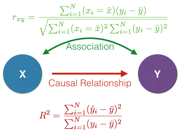
The hypothesized relationship between the two variable sets determines which kind of model to assume.