34 Niche Modeling

install.packages(c("rJava","dismo"))
library("rJava")
library("dismo")

Some of the more common approaches used to characterize a niche is through the use of either logistic regression approaches or maximum entropy. At present, the implementation of the latter appoach, dentoed as MaxEnt, is widely used and will be highlighted in this section. For you to use this, you need to Download the java interface for MaxEnt. You will have to sign in to download the files. Use the .zip archive for this, it has all the files you need. This is not the GUI interface, it is only the underlying java machinery the GUI uses. On some platforms, you may also need to download the legacy Java runtime (as of the writing of this it was SE 6) for your computer to run the analysis. The underlying analyses are done in Java and only accessable to R using this approach.

Unzip those files and put each of them in the directory defined by the following command:

system.file("java", package="dismo")

## [1] "/Library/Frameworks/R.framework/Versions/3.3/Resources/library/dismo/java"

This puts the java executables into a directory within dismo. This allows the dismo functions to use the latest version of maxent directly. To get started, allow the java executables to access up to 1Gig of your RAM by setting the following option prior to loading in dismo

options(java.parameters = "-Xmx1g" )
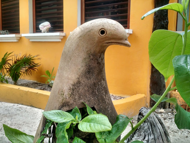
library(dismo)

Now we can get to work. In this example, I’ll use biolayers found to be informative for the distribution of Euphorbia lomelii (Euphrobiaceae), the host plant for Arapatus attenuatus that we collected from both observations and all available herbarium specimen records that had sufficient spatial specificity.

I load these in using the raster() function. These rasters have already been cropped to the extent enclosing all the arapat populations (as in 31.1). I have these stored in a subdirectory called ‘spatial_data’ and load them in as a RasterStack object (a set of rasters).

library(raster)
files <- c( "bio2.tif", "bio7.tif", "bio8.tif", "bio13.tif", 
            "bio15.tif", "bio17.tif")
files <- paste("./spatial_data",files,sep="/")
bio_layers <- stack(files)

Next, I load in the spatial coordinates of the recorded sites of known occurrence. I set aside 20% of the observed sites to use as a test of the model we derive.

sites <- read.csv("./spatial_data/EuphorbiaAllLocations.csv",header=TRUE)
num_train <- round(nrow(sites)*.8)
idx <- sample( 1:nrow(sites), size=nrow(sites), replace=FALSE )
pts.train <- sites[ idx[1:num_train] , 2:3]
pts.test <- sites[ idx[ (num_train+1):length(idx)], 2:3]
c( Train=nrow(pts.train), Test=nrow(pts.test) )

## Train  Test 
##   301    75

The maxent model itself is used determine the extent to which site-specific factors may be able to predict the presence of this species.

fit <- maxent(bio_layers,pts.train)

The html output from the analysis can be viewed in your default browser by showing the model.

fit

Which produces output that looks something like the following inset.

Here are some quick ways to view and interpret output from the maxent approach.

plot(fit)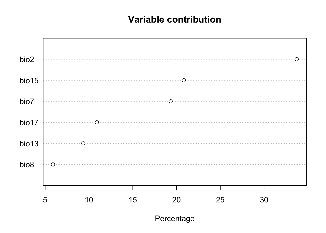

response(fit)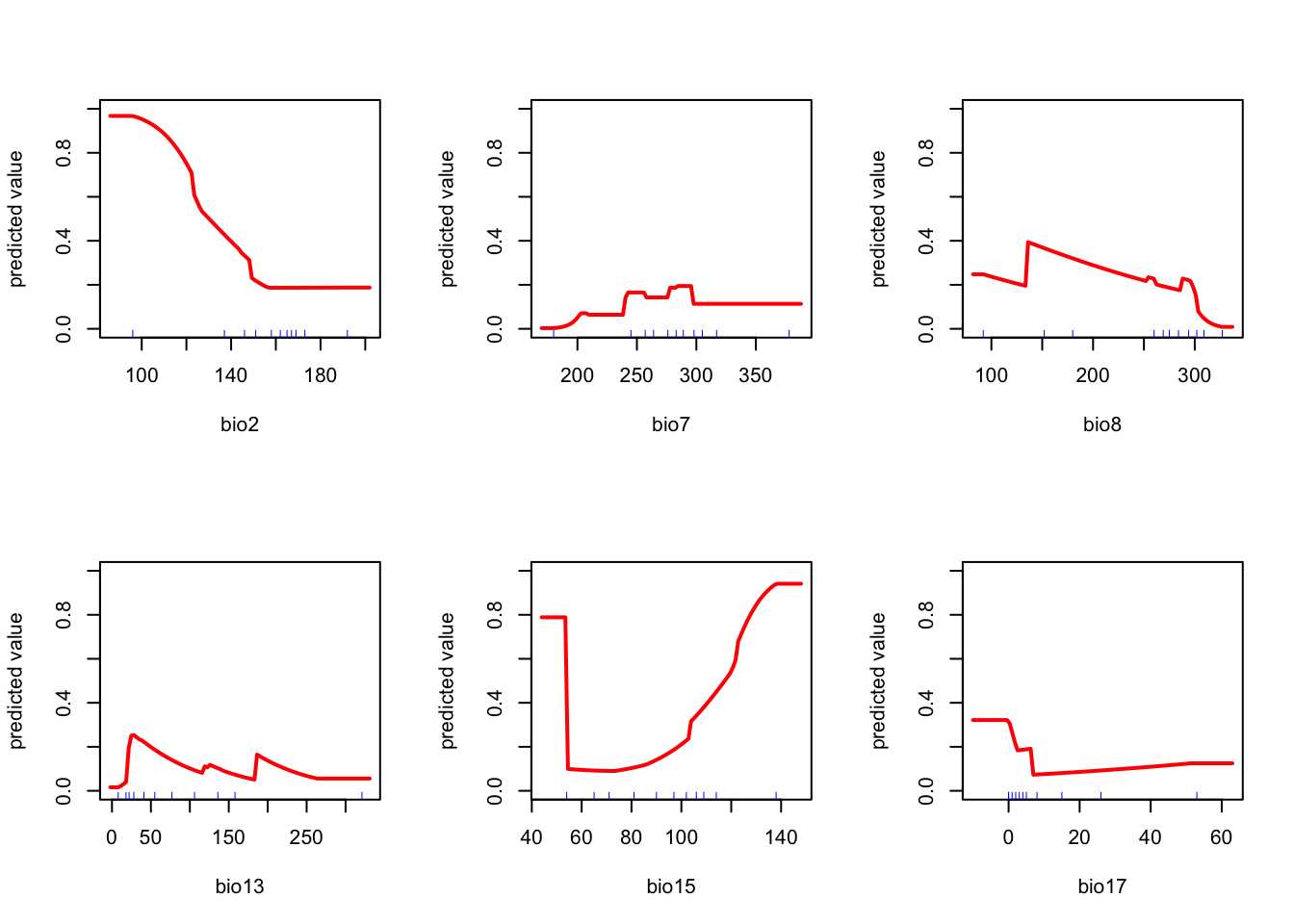

r <- predict( fit, bio_layers )
plot(r, xlab="Longitude",ylab="Latitude")
points( pts.train, pch=3, cex=0.75)
points( pts.train, pch=16, cex=0.75)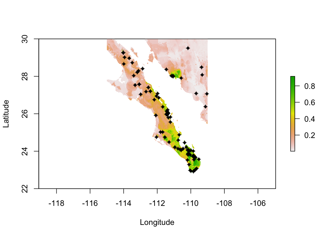

pts.random <- randomPoints(bio_layers, 1000)
fit.eval <- evaluate(fit, p=pts.test, a=pts.random, x=bio_layers)
fit.eval

## class          : ModelEvaluation 
## n presences    : 75 
## n absences     : 1000 
## AUC            : 0.92898 
## cor            : 0.5514523 
## max TPR+TNR at : 0.6826505

vals.pred <- data.frame( extract( bio_layers, pts.test) )
vals.rand <- data.frame( extract( bio_layers, pts.random) )
fit.eval_rnd <- evaluate(fit, p=vals.pred, a=vals.rand)
fit.eval_rnd

## class          : ModelEvaluation 
## n presences    : 75 
## n absences     : 1000 
## AUC            : 0.92898 
## cor            : 0.5514523 
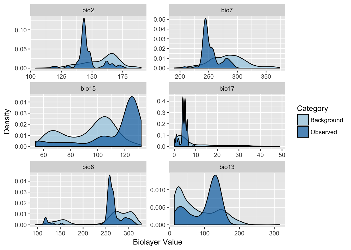
## max TPR+TNR at : 0.6826505

library(ggplot2)

df <- data.frame( Val=NA, BioLayer=NA, Category=NA )

layers <- names(vals.pred)
for( layer in layers){
  Val <- c( vals.pred[[layer]], vals.rand[[layer]] )
  Category <- c( rep("Observed",nrow(vals.pred)), rep("Background",nrow(vals.rand)))
  df <- rbind( df, data.frame( Val, BioLayer=layer, Category))
}
df$BioLayer <- factor( df$BioLayer, ordered=TRUE, 
                       levels = names(vals.pred)[c(1,2,5,6,3,4)])
                                                                              

df$Category <- factor( df$Category )
df <- df[ !is.na(df$Val),]
p <- ggplot(df,aes(x=Val, fill=Category)) + geom_density(alpha=0.75)  
p <- p + facet_wrap(~BioLayer, nrow=3, scale="free") 
p <- p + scale_fill_brewer(type="qual",palette=3) 
p + xlab("Biolayer Value") + ylab("Density")